
A View of the Terms and Agreements: Reading Big Tech Privacy Policies at a Distance
With our class having recently discussed our collective frustration and ignorance toward the terms and conditions of “Big Tech” companies, I felt it worthwhile to take a look at the privacy policies of major technology corporations — and some of their subsidiary digital platforms — in not only the United States, but also China. Part of my reasoning behind this international perspective on the tech sector draws from an interest in probing at some of the similar and disparate ways in which major American and Chinese tech companies articulate their terms and conditions regarding the management of user privacy and personal data. At the onset of my project, I didn’t necessarily have a concrete grasp on what sort of trends I expected to find, but I also felt as though this uncertainty might lend itself to a few hidden insights given that I to some extent let the data do the talking. Situating myself in the playful spirit of to “the hermeneutic of screwing around,” vis-a-vis Stephen Ramsay, I wanted to poke around inside of these deconstructed corporate texts, to unravel their legalese and consolidate it into a dataset, picking and prodding at trends in their diction, syntax, and structure. Meanwhile, I thought it important to keep an eye out for subject matter that might have otherwise gone unacknowledged by 91% of users when checking the proverbial box: the vast majority of us consumers who at the mere sight of these ghastly documents choose to throw our arms in the air before abruptly agreeing to the terms and conditions.
In the spirit of normalizing failure and learning from past mistakes, I’d like to note that my ambition exceeded my grasp when first gathering text corpora for this project, if only because I started by compiling data on individual privacy policies and service agreements from Amazon, Facebook, and Twitter, as well as Alibaba, Sina Weibo, and WeChat. This entailed that I gather twelve total files for text analysis in Python. I intended to analyze each file for three specific linguistic measurements — term frequency, bigram frequency, trigram frequency — which, as far as Excel columns go, meant multiplying twelve times six due to the fact that each corpus requires three columns for its key (e.g. “privacy, notice”) and three columns for its value (e.g. “9”) Suddenly the number of columns of data in my spreadsheet ballooned to 72, which of course is too much data for one person to qualitatively parse in a limit time span. Needless to say, I had some reflecting to do.
In writing code to preprocess these text files, I decided to clean house on punctuation, uppercase characters, as well as integers. These alterations are not without ambivalence. Indeed, I think there are salient insights hidden among the use of numbers across these corpora. For one, these documents are written in a legal register that so happens to self-reference numbered sections with its own set of terms and conditions, disclosed earlier or later in a given document. While robust on a legal level, this technique doesn’t exactly enhance readability despite the fact that these documents are explicitly meant for consumers who must in turn agree with its obtuse parameters. In any case, these documents don’t self-reference themselves via numbered sections so often that it becomes a problem solvable by means of computational analysis, so I decided to table that line of thinking for another day. What’s more, I decided to import and apply NLTK’s stopword dictionary to remove from each corpus certain prepositions and conjunctions, which would otherwise convolute bigram and trigram data.
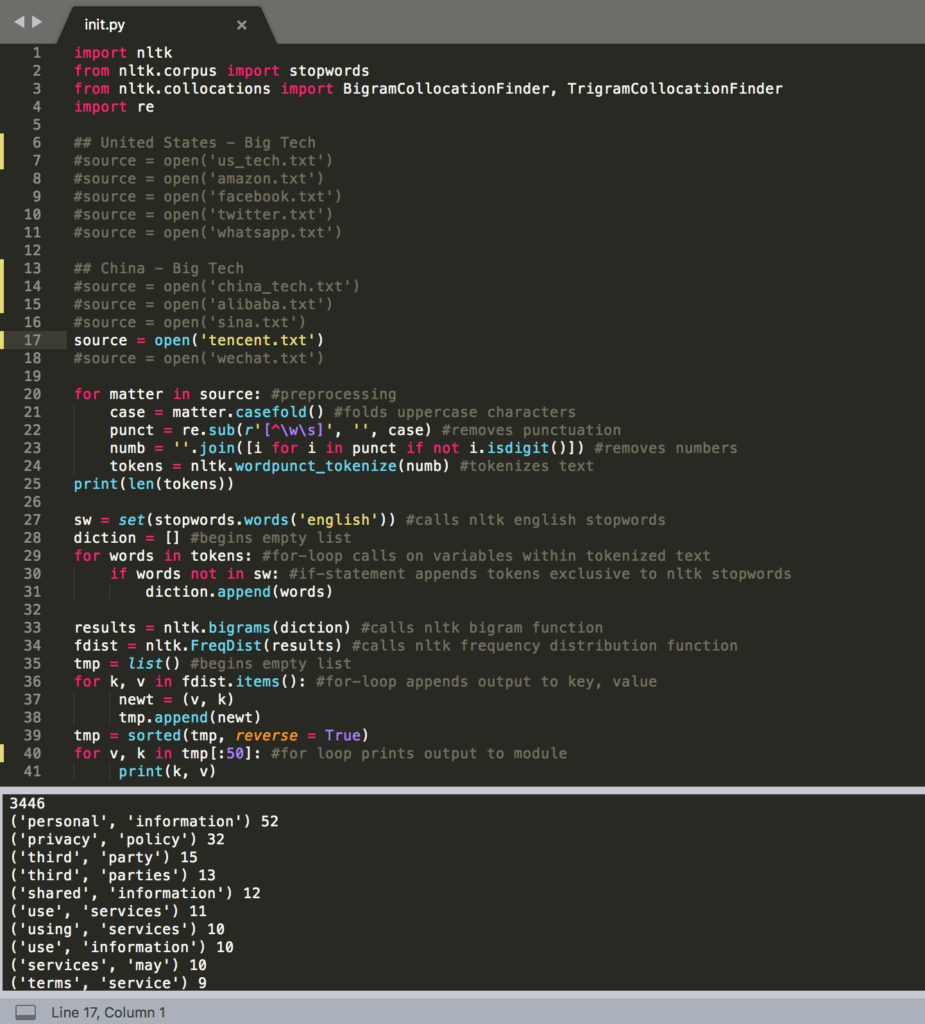
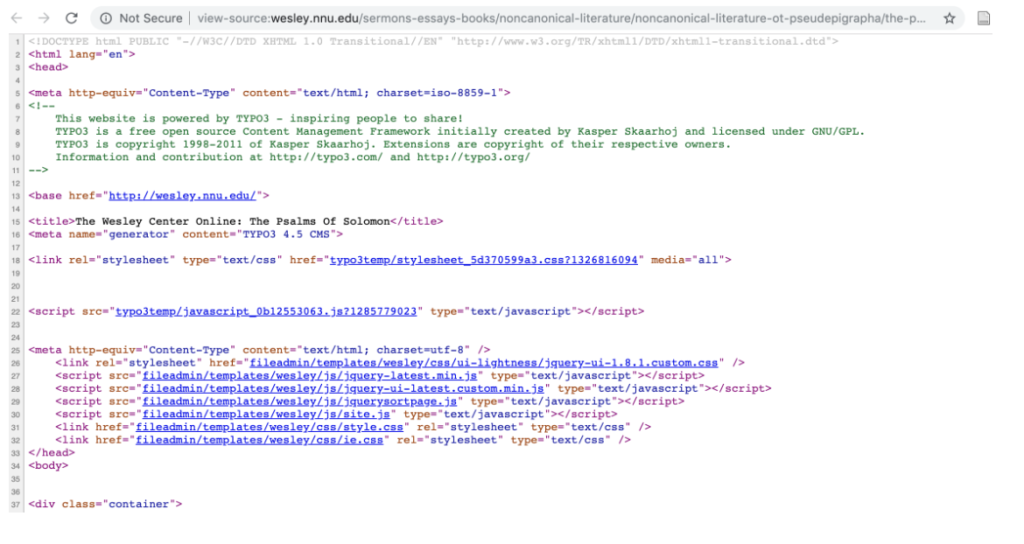
For the sake of transparency, I’ve taken a screenshot of the code I used to retrieve high frequency words, bigrams, and trigrams throughout each corpus. To shift between these three measurements only required that I reassign the identifiers to certain variables, while moving between corpora required that I remove the commented-out code preceding the call to open each file, as with line 17.
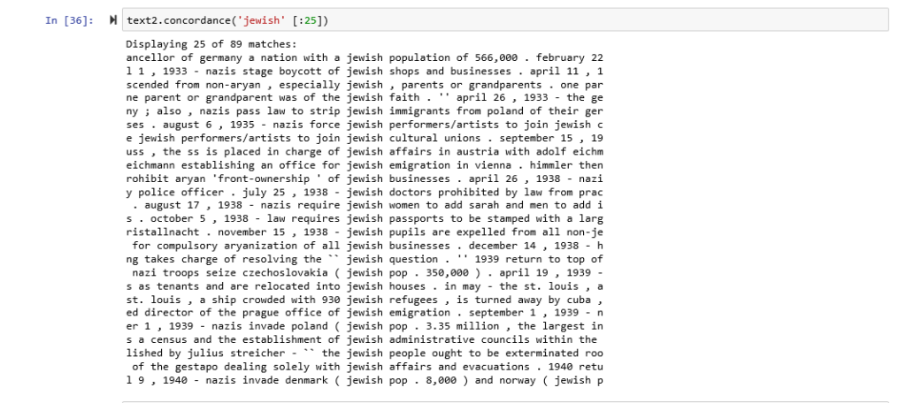
Once I migrated the results for each corpus over to Excel, which took longer than I would like to admit, I started probing for patterns between two or three relative datasets but mostly between analogous companies vying for a constituent market, as well as between American and Chinese companies and their subsidiaries. Comparing WhatsApp and WeChat struck me as promising in that either company is a subsidiary application of a much larger multinational conglomerate, both vying to keep their share of the mobile communications market. When first surveying this data, I came to the realization that these privacy policies were not necessarily long enough on their own to yield insightful statistical results. But that isn’t to say they weren’t informative, because they most certainly were. Pulling trigram frequency from the privacy policies for WhatsApp and WeChat alone seemed to me a far more revealing experience than colloquially skimming these documents could ever be. I was struck right away, for one, by the bare repetition by both apps to emphasize the importance of understanding the effect of third-party services on information security. Note, however, that the emphasis is by no means unique to WhatsApp and WeChat: there are 170 total occurrences of ‘third-party’ across my full dataset when the term is normalized into a single word without permutations.
| WhatsApp Privacy Policy | WeChat Privacy Policy | ||
| Sum length: 3489 | Sum length 5019 | ||
| Trigram | Count | Trigram | Count |
| facebook, company, products | 7 | legal, basis, eu | 18 |
| understand, customize, support | 6 | basis, eu, contract | 14 |
| support, market, services | 6 | tencent, international, service | 6 |
| provide, improve, understand | 6 | wechat, terms, service | 5 |
| operate, provide, improve | 6 | understand, access, use | 5 |
| improve, understand, customize | 6 | better, understand, access | 5 |
| customize, support, market | 6 | access, use, wechat | 5 |
| third-party, services, facebook | 5 | third-party, social, media | 4 |
| third-party, service, providers | 5 | provide, personalised, help | 4 |
| services, facebook, company | 5 | provide, language, location | 4 |
| use, third-party, services | 4 | privacy, policy, applies | 4 |
| operate, provide, services | 4 | personalised, help, instructions | 4 |
Perhaps the most noteworthy difference between either app’s privacy policies appears lie in the textual space that WeChat dedicates to covering the legal bases of the European Parliament. (Note: the dataset cites them as “legal basis” as a difference in convention.) Inaugurated with the “The Treaty on the Functioning of the European Union” in 2007, these legal bases more specifically enable the EU precedent to conduct legal action and legislate policy on the grounds of certain predefined issues across Europe. In the WeChat privacy policy, references to “legal bases” follow a section heading on the management of user data, written in an effort to meet specific cases of European international law on personal privacy. Here’s how that section begins, with an example of its subsequent content:
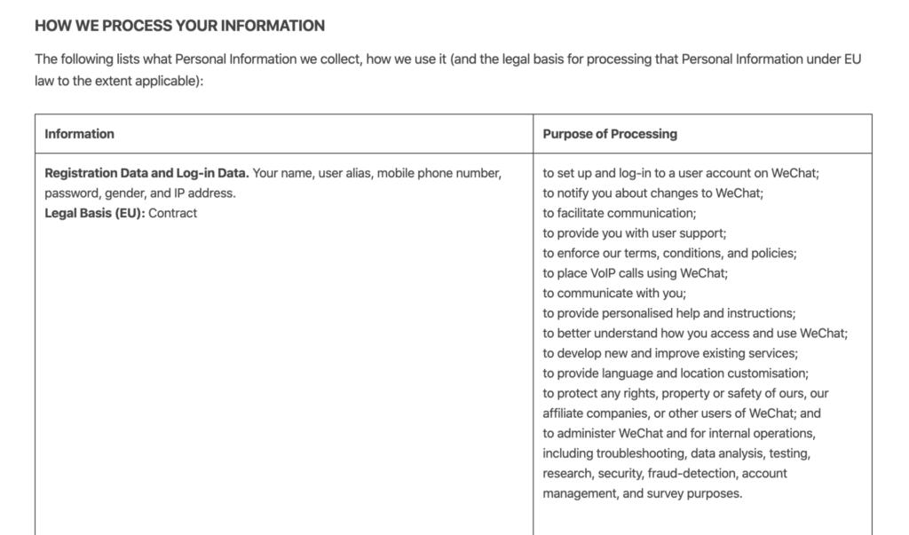
While I don’t claim to be making any fresh discoveries here, I do think it’s interesting to consider the ways in which WeChat qualifies its international link to the EU legal bases by hedging EU protocol with the phrase: “to the extent applicable.” While appearing to satisfy EU legal bases as far as international jurisdiction applies, in other words, WeChat seems to permit itself a more flexible (if vague) standard of privacy for individuals who partake in its services outside the reigns of the European Union. This begs the question of where specifically American users factor into the equation, not to mention whether or not EU-protected users are safeguarded when their personal data crosses international boundaries by communicating with users in unprotected countries. Likewise, another question involves how this matter will impact the U.K. once they’ve successfully parted ways with EU on Jan 31, 2020. Namely, will the legal ramifications of Brexit compromise user data for British citizens who use WeChat? What of applications or products with similar privacy policies as WeChat? Scaling this thread back to Tencent, I was somewhat surprised to find little to no explicit mention of the EU in the top 30 word, bigrams, and trigrams. However, I did notice that tied for the 30th most frequent bigram, with four occurrences, was “outside, jurisdiction.” Searching through the unprocessed text document of Tencent’s privacy policy, this bigram led me to a statement consistent with the WeChat’s focus on EU legal bases, excerpted below. (Bolded language is my own.)
You agree that we or our affiliate companies may be required to retain, preserve or disclose your Personal Information: (i) in order to comply with applicable laws or regulations; (ii) in order to comply with a court order, subpoena or other legal process; (iii) in response to a request by a government authority, law enforcement agency or similar body (whether situated in your jurisdiction or elsewhere); or (iv) where we believe it is reasonably necessary to comply with applicable laws or regulations.
So, while EU legal bases play no explicit role in the multinational’s broader privacy policy, such legal protocol nonetheless seems to play a role, though again only when relevant — or, at least in this case, “where [they] believe it is reasonably necessary to comply applicable laws or regulations.” It was at this point that I started to consider the vast array of complexity with which multinational conglomerates like Tencent compose primary and secondary privacy policies in an effort to maximize information processing while also protecting their company and its subsidiary products from legal action. In turn, I began to consider new and more focused ways of examining these privacy policies in terms of their intelligibility/readability as textual documents.
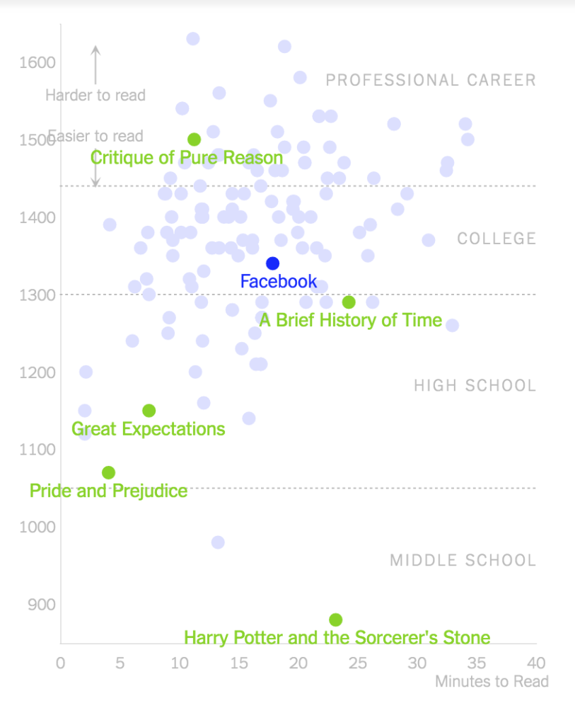
This question led me to discover the following NYT article by Kevin Litman-Navarro on privacy policies written by major tech and media platforms that “opaquely establish companies’ justifications for collecting and selling your data” with their difficulty and verbosity of language. Using the Lexile test to determine a text’s complexity, Litman-Navarro analyzes a flurry of some odd 150 privacy policies, some of which are included in my dataset, such as Facebook, which his evaluation determines to be somewhere between The Critique of Pure Reason by Immanuel Kant (most difficult) and A Brief History of Time by Stephen Hawkings (more difficult) in its range of readability. Meanwhile Amazon’s privacy policy, whose word count totaled at 2624 as opposed to Facebook’s heftier 4203 words, was between A Brief History of Time and Great Expectations by Charles Dickens.
| Privacy Policy | Lexical Diversity |
| 5.598529412 | |
| 5.237951807 | |
| 5.120921305 | |
| 5.027633851 | |
| Alibaba | 4.779365079 |
| Tencent | 4.627151052 |
| Amazon | 4.276679842 |
| Sina Weibo | 3.184115523 |
In an attempt to replicate a similar sense of these results, I employed NLTK’s measurement of lexical diversity and recorded my statistical results to the right. If lexical diversity is any indication of readability, then it seems as if these results reflect part and parcel of Litman-Navarro’s analytics, with Twitter indicating a higher diversity index than Facebook, which in turn indicates a higher diversity index than Amazon.
Considering the size of my dataset, I think moving forward it might be best to simply link it here for those who are themselves interested in interpreting the qualitative results of these privacy policy texts. Ultimately, I see my project here as the groundwork for a much large, more robustly organized study of these legal documents. There’s tons and tons of data to be unearthed and analyzed when it comes to the microscopic trends of these legal documents, particularly when placed against the backdrop of a much grander scale and sample size. Whereas I’ve picked my corpora on a whim, I think a more cogent and thoroughgoing inquiry into these documents would merit hundreds of compiled privacy policies from tech and media companies across the world. A project worth pursuing someday soon indeed…
Looking for Parallels of Imperialism: Manifest Destiny | Generalplan Ost.
For my text analysis project, I decided to build two corpora each based on a political doctrine of imperialism.
This is the first text analysis project I’ve undertaken so I want to make clear that the goal of this analysis is experimentation. I am not attempting to draw any finite conclusions or make general comparisons about the historical events which give context to these corpora. The goal is to explore the documents for topical parallels and reciprocity of language simply based on the texts; and hopefully have some fun while discovering methods of text analysis. Nonetheless, I am aware that my selection process is entrenched in biases related to my epistemological approach and to my identity politics.
When I began this project, I was thinking broadly about American Imperialism. I was initially building a corpus for exploring the rise of American imperialism chronologically starting with the Northwest Ordinance to modern day military and cultural imperialism through digital media. The scope of the project was simply too massive to undertake for this assignment, so I started thinking more narrowly about Manifest Destiny. I started thinking about the Trail of Tears, and as I did, my mind went back and forth to parallels of the Death Marches in Nazi-Occupied Europe. So I thought; why not build two corpora to reflect the two imperialist doctrines which contextualize these events. Manifest Destiny and Generalplan Ost.
Manifest Destiny Corpus
The following bullet points are the notes that best sum up my selected documents for Manifest Destiny.
- U.S Imperialist doctrine of rapid territorial expansion from sea to shining sea.
- Territorial expansion will spread yeoman virtues of agrarian society
- Romanticization of rugged individualism on the frontier
- Removal and massacre of inhabitants of desirable lands.
- Racial superiority over native inhabitants.
- Territorial expansion is intended by divine Providence.
Generalplan Ost Corpus
The following bullet points are the notes that best sum up my selected documents for Generalplan Ost.
- German Imperialist doctrine of rapid territorial expansion across Eastern Europe.
- Territorial expansion will create an enlightened peasantry
- Romanticization of nationalistic racial purity as patriotism
- Deportation and genocide of inhabitants of desirable lands.
- Racial superiority over Jews, Slavs, Roma, and non-Aryans.
- Territorial expansion is justified by WWI’s illegitimate borders.
Building the corpora
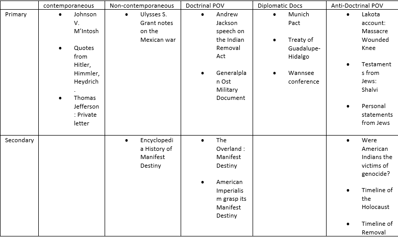
Building the corpora was one of the most time-consuming processes of the analysis. Prior to selecting my documents, I identified some important criteria that I felt were necessary for a balanced representation of voices. I wanted to incorporate both doctrinal and anti-doctrinal perspectives, both primary and secondary sources, as well as temporal distance in the categories of contemporaneous and non-contemporaneous. I used a triage table to sort documents. Here are a few examples;
Once I had selected ten documents for each corpus, I was faced with what seemed to be the insurmountable task of tidying the data. Several documents were in German. I had all types of file objects, some web-pages, some PDFs, and some digitized scans. For the digitized scans which were mostly diplomatic documents, I was able to find a digitized text reader from the Yale Law Avalon Project which not only read the texts but translated them from German to English since it already had a matching document in its corpus. For the secondary source German document, I used the “translate this page” web option. I scraped all the web-pages using BeautifulSoup and converted all my documents into plain-text files for both corpora. By the end of my second day on the project, I had created 20 files on which to run some text analysis.
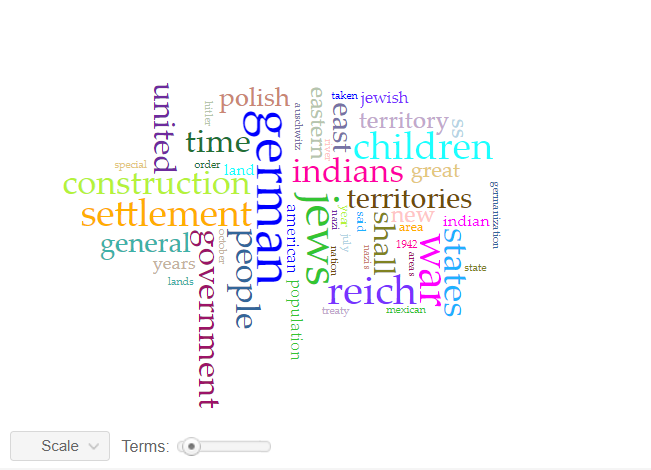
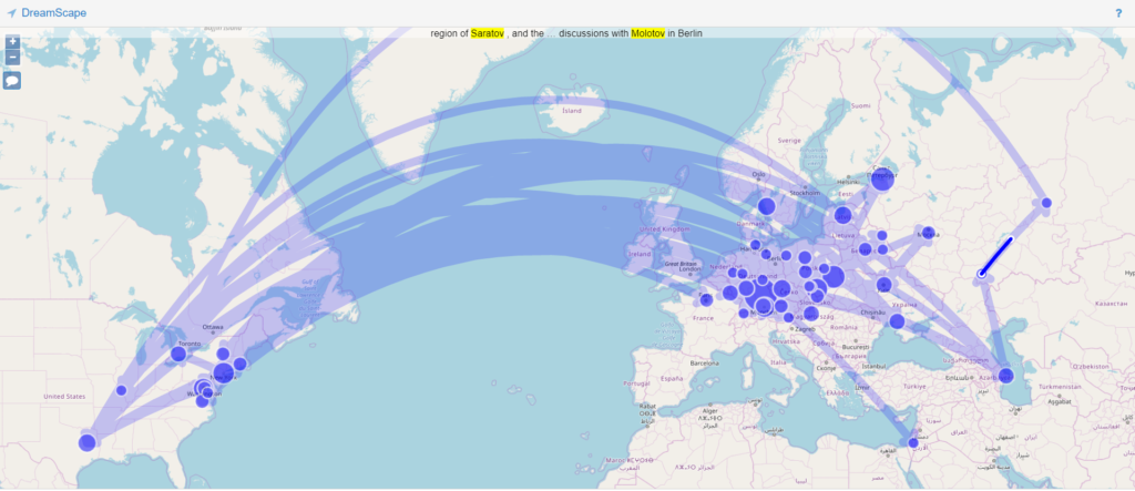
I was a bit nervous about building my own python notebook, so I started working with Voyant. At first, I uploaded each corpus into Voyant to analyze one by one. Not yet looking for parallels, I wanted to see what a distant reading of the selected documents would look like on their own. And immediately after loading my Generalplan Ost corpus, I was greeted with five mini windows of visualized data. The most remarkable one was the word cloud with terms such as; Reich, German, Jews, 1941 colorfully appearing in large fonts, indicating the lexical density of each term in the corpus. Similarly, with the Manifest Destiny corpus, terms such as; War, Indian, States, Treaty also appeared in a constructed word cloud. I found many interesting visualizations of the lexical content of each corpus, but my goal was to bring the whole thing together and search for parallels in topics and reciprocity in the language.
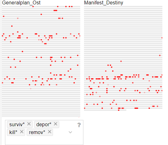
I brought the two corpora together and started digging. One of the best tools I found on Voyant is the MicroSearch tool which displays a selected term in its local occurrence (where it is found) over the entire corpora. It displays lexical density in context as a miniaturization of the original text format and not as an abstract visualization. It is tantamount to geotagging items on a map. You can look at the map and see where each item is located in relation to other items. I found this tool incredibly effective at displaying parallels across corpora. For example, in this MicroSearch capture, I was looking for the terms with the following root words (surviv*, deport*, kill*, remov*) indicated by (*). The MicroSearch returned all instances of all words with the roots I selected wherever they were found. As a result, I was able to visualize a key topical parallel in the corpora; the term removal being frequent in relation to Indian, and the term deportation being frequent in relation to Jewish.
This capture is a MicroSearch of the terms with the following root words (terri*, empi*, imperi*, land*, settl*, colon*, constr*)
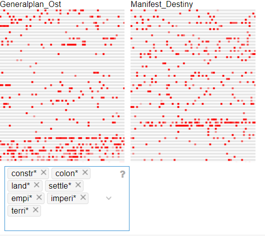
If I were to group these root words into the topic of ‘imperialism’. I could make the case for a topical parallel based on the lexical density and distribution of those terms in the corpora.
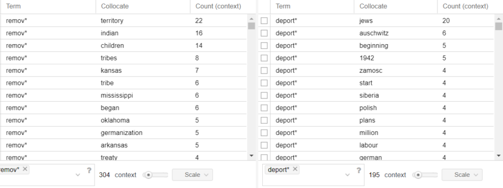
Another tool that I found useful was the collation tool. The collation tool matches words that repeatedly appear next to each other and counts the frequencies at which they occur. Matching two words allows for each word to frame the context of the other and the higher the frequency number, the stronger the relationship is between those words. For example, in this capture, the term deport* and the term Jews are found together 20 times. Whereas the term remov* and the term Indian occur together 16 times.
The crossing bars in the trend graph represent a reciprocal relationship between the terms Jew: Indian. The term Jew* appears 306 times in the Generalplan Ost corpus which is comprised of 45495 tokens. I can determine the numerical value of its lexical density as follow; 306/45495 = 0.00672601 which in percentage equals 0.673%
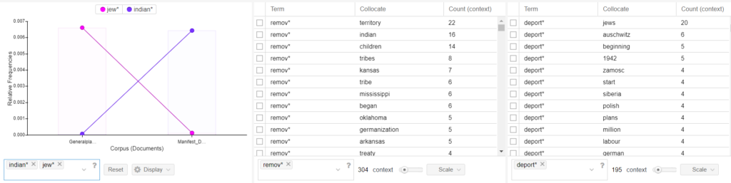
The term Indian* appears 257 times in the Manifest Destiny corpus which is comprised of 39450 tokens. 257/39450 = 0.00651458 which in percentage equals 0.651%.
While I experimented with Voyant, I became aware of the limitations of its tools. And I started to think about building a python notebook. I was hesitant to do so because of my limited use of python and the complicated syntax that easily returns error messages which then takes extra time to solve. Despite my hesitance, I knew there was much more in the corpora to explore and after spending an hour parsing through the notebook with Micki Kaufman, I felt a little empowered to continue working on it. The first hiccup happened in the second line of code. While I was opening my files, I ran into an UnicodeEncode error which was not a problem for a web-based program like Voyant. I had saved my German texts using IBM EBCDIC encoding. I had to go back and save everything as UTF8. It took me reading about a chapter and a half of the NLTK book to figure out that I could not do a text concordance, or a dispersion plot from a file that was not a text.text file. But once I was able to learn from those errors, I was excited at the possibility to discover so much more using python.
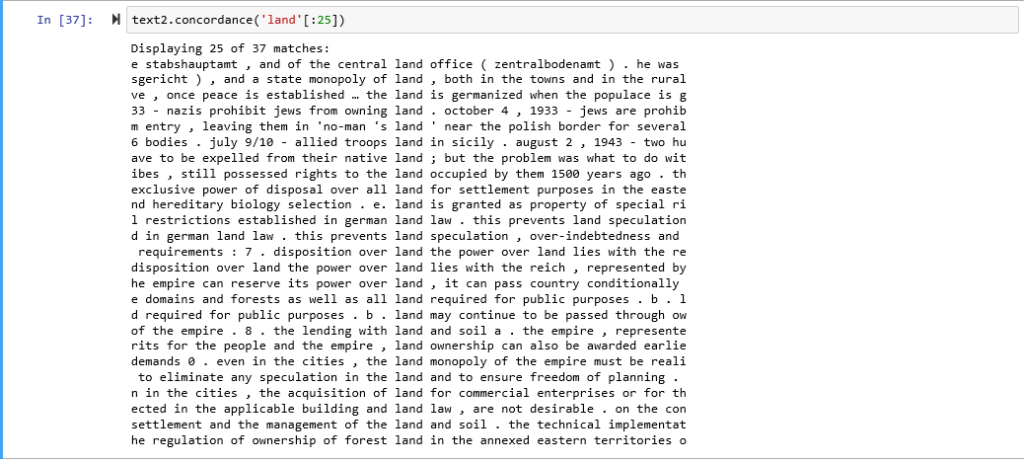
Here I created a concordance with the Generalplan Ost corpus for the word; land
(A text concordance centralizes a selected term within a text excerpt that surrounds it to give context to the term.)
Look at the key words surrounding the word land in this instance.
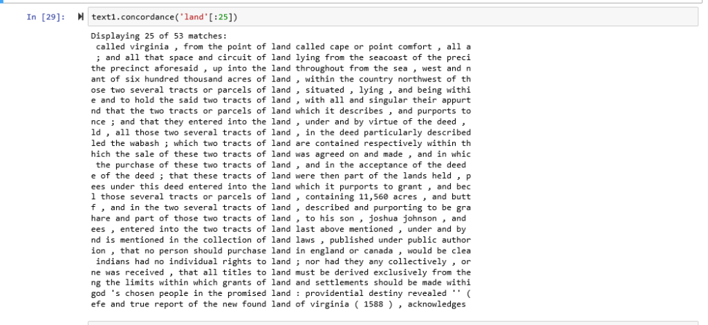
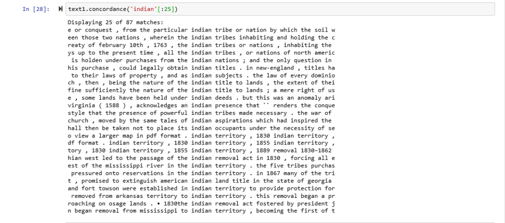
Here I created a concordance with the Manifest Destiny corpus for the word; land
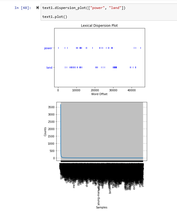
Here I created a dispersion plot with the Generalplan Ost corpus for the words; power: land

Here I created a dispersion plot with the Manifest Destiny corpus for the words; power: land
Here are concordances for the terms Jewish: Indian
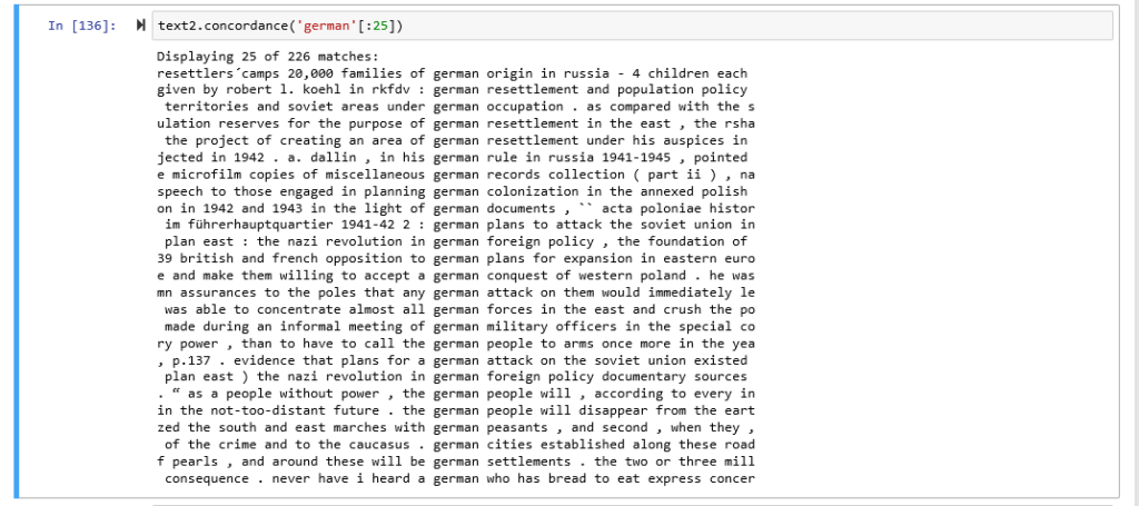
Here are concordances for the terms American: German

Although I can enumerate many parallels in the corpora. There were some distinct differences that I found.
For example, in Voyant, words that appeared in large fonts in the word cloud in the Generalplan Ost corpus such as Reich and German, and to a lesser degree Hitler and Himmler were highly correlated to the doctrinal perspective which makes me think that in spite of my efforts at representing as plural a selection of voices as I could find, the documents I selected for their contextual importance still overwhelmingly represented the doctrinal perspective. In the Manifest Destiny corpus, I noticed that words such as; war, Indian, states, and shall, were the most frequently distributed. I wonder if United States being two words instead of one and being often abbreviated to U.S or America contributed to a lexical density split. In addition, the Manifest Destiny corpus beside having the same number of documents as the Generalplan Ost corpus contained 6, 045 fewer tokens.
Here are some general data from my python notebook
| Corpus | Total tokens | Unique tokens | Lexical density % | Most unique words |
| Manifest Destiny | 39450 | 6201 | 13.80% | Indian, treaty, Mexican, destiny, deed |
| Generalplan Ost | 45945 | 6216 | 12.05% | Reich, polish, ss, germanization, 1942 |
Here are some additional captures from Voyant and python that are also interesting.


Rap albums, sorted by the size of their vocabulary.
A few years ago, I came across Matt Daniels’ study on rappers, ranked by the size of their vocabulary. The study regularly is updated throughout the years, to take into account of newer artists, or new albums artists have released. Being a fan of this visual essay, along with being a fan of modern rap, I wanted to center my praxis assignment as a smaller-scale version of the study: the top five rap albums of the past year, sorted by the size of their vocabulary.
I decided to visit Billboard to choose the top five albums. Although we are approaching the end of 2019, the franchise did not scale rap albums for the year. I looked to 2018’s top rap albums, which (in order) are Drake’s Scorpion, Post Malone’s beerbongs & bentleys, Cardi B’s Invasion of Privacy, Travis Scott’s Astroworld, and Post Malone’s other album, Stoney. To locate lyrics, I chose Genius. Unlike other lyric sites like Metrolyrics or AZlyrics, many artists directly contribute their lyrics to this site. Additionally, the site also serves as a community, in which both artists and listeners can select verses from lyrics and annotate and interpret rappers’ play on words, disses to other artists, and their overall, unique rhetoric.
I decided to use Voyant, as I wanted to document each album’s number count of unique words, a term used in the original study– in which multiple presentations of the same word is counted once. Admittedly, I had to blush once I had uploaded the lyrics to one song–to find expletive words profoundly appear on Voyant’s cirrus. To make the assignment appropriate, I have ranked the same five albums, based on its unique word forms, with its corresponding album covers.

Scorpion, Drake
10,095 total words
1,745 unique word forms
25 Tracks

Invasion of Privacy, Cardi B
7,727 total words
1,418 unique word forms
13 Tracks

ASTROWORLD, Travis Scott
5,710 total words
1,244 unique word forms
17 Tracks

beerbongs & bentleys, Post Malone
8,707 total words
1,178 unique word forms
18 Tracks

Stoney, Post Malone
6,814 total words
983 unique word forms
14 Tracks
Initially, I was excited to drop Genius URLs directly into Voyant’s field box and quickly collect data. However, I soon realized Voyant collected all text from the site– including the site’s header, breaking text such as [Chorus], [Verse 1], [Bridge], usernames on the side, annotations and supplemental articles listed to the side of the lyrics. To create a more accurate word count, I created a Google document for each album, and copied and pasted the lyrics directly there. Doing so also helped with slimming down the text, as there were many featured artists and sampled artists that I did not want to inflate the primary artists’ unique word count. I then selected the entire text of each document into Voyant, and I immediately collected the unique word count of each album. Overall, Voyant was a straightforward guide for this assignment, but my learning lesson here was the importance of organizing the data first, as it was tempting to drop the links to each lyric on the field box, but only to collect inaccurate word counts.
Looking back now, I would have liked to explore this same project in my own form of a data visualization. Granted, many of the lyrics are inappropriate to discuss in an academic setting, and I am a bit embarrassed to share the Voyant links of my album documents, but there are other ways to present data.
I strongly appreciate Daniels’ visualizations for his essay, in which he presents an image of the rapper, and from the motion of the cursor, viewers can discover each of their metrics. I plan to render a a data set similar to this, one day.

Mapping an education textbook against its syllabus
My primary goal for this assignment was to learn Voyant’s functionality, but I also wanted to understand how I might be able to use it in my current work. Over the past year I have supported faculty members at Hostos Community College who are building textbooks with Open Educational Resources (OER). Most of the faculty I have supported need assistance finding appropriate content or a satisfactory amount of content for their texts. They often get through 50-75% of the book on their own, and then need help identifying openly licensed content for gap areas or help identifying chapters that are sparse. I wondered if it would be helpful to faculty to create a corpus for the complete book and each chapter of their book, and then compare to their syllabus or course objectives.
For the sake of this assignment I chose to use a textbook for EDU 105: Social Studies for Young Children, one on which I am currently working. I decided to look at how the text of the syllabus — which included course objectives and weekly topics — compared to the content of the course material the professor wrote. To do so, I created one corpus of content for the textbook — with each section a separate document — and one corpus for the syllabus. For each I copied and pasted content from their respective websites (the books are built in LibGuides and syllabus is in Google Drive) into the “Add Texts” window on the home page. I found it very usable and straightforward.
Here is a view of the textbook corpus with the default dashboard:

(https://voyant-tools.org/?corpus=883399c79d0ce541ce9dad5c5eb0fec4)
Here is a view of the syllabus corpus with the default dashboard:

(https://voyant-tools.org/?corpus=6c93088ad815d60fab77b9d63e02f659)
I primarily looked at the “cirrus” word cloud, term count, and links tools for my review, and asked the following questions:
- What are the most visually prominent words (based on term frequency in the content), and do they give me an idea of what the class covered?
- Textbook: Overall I would say that it did, but I needed to use a combination of tools for the complete picture. While the “cirrus” world cloud gave me a quick visual on the most common words, I could not create two-word phrases, like social studies or early childhood. “Social” and “Studies” were separate, so it wasn’t obvious that the class was about social studies. However, when I looked at the terms tool, I could see “social” and “studies” stacked together. As the second and third most common words. I could also see the link between “social” and “studies” with the link tool. Early Childhood did require that I scroll down through the list to understand that the course was for teachers of younger children, but I understood enough of what the course was about. I would say that the links tool was the best reflection of the class content (see image below).
- Syllabus: Regardless of the tool, the syllabus could have been appropriate for most courses. However, if this syllabus was compared to a syllabus for a course outside of the Education department, it is likely that it would be evident that it was for an education course.
The Summary tool was actually a good complement to the visual tools, because I was able to see the most frequent words (social, studies, students) and distinctive words per document (chapter).

- Did the scope of terms in the textbook content match the syllabus?
- The textbook terms covered all of the identified topics and goals in the syllabus, and was more specific. I found the Terms tool to be most helpful for this comparison, but once I realized that Voyant wasn’t great with the syllabus I actually compared the visualization for the textbook to the syllabus word document outside of Voyant.
- I hoped that comparing these two would show gaps in the content, but none of the tools I used helped with this evaluation.
- Are any chapters more content-rich than others?
- The Reader and Summary tools was superficially helpful for this. For example, the Reader tool showed a colored bar per document, so I could see which documents (in my text these are chapters) had more words. The Summary tool counted the number of words.
- This would not work for pages with a number of links to websites with additional reading, nor would it work for other media, like videos and images, which this textbook included.
I intent to continue exploring the following:
- How can I exclude what I consider to be false results? By this I mean common terms in all documents but distract from what I am reviewing? This is beyond stop words.
- Can I hide and reveal documents to compare subsets, or do I need to create a different corpus for each grouping?
- Would the visualizations change if I flattened multiple documents into one as opposed to multiple documents?
- Is it possible to see the syllabus and the textbook documents in parallel in the same screen?
Analyzing American Cookbooks
Like many people around this time of year, I am faced with the decision of what to make for Thanksgiving. Recipes, traditional and modern, fill my brain as I decide what my guests will accept in their holiday meal. Recent conversations about my recipes have made me think about the history of American cooking, so I thought for this assignment I would look at American Cookbooks to see what were popular ingredients and cooking methods during our nation’s early history.
I used Michigan State University’s Feeding America Digital Project (https://d.lib.msu.edu/fa) to find cookbooks published in America and written by American authors. The site has 76 cookbooks from the late 18th century to the early 20th century and offers multiple formats to download. I used seven cookbooks from 1798-1909:
- American cookery by Amelia Simmons (1798)
- The frugal housewife by Susannah Carter (1803)
- The Virginia housewife: or, Methodical cook by Mary Randolph (1838)
- The American economical housekeeper, and family receipt book by E. A. Howland (1845)
- The great western cook book: or, Table receipts, adapted to western housewifery by Anna Maria Collins (1857)
- The Boston cooking-school cook book by Fannie Merritt Farmer (1896)
- The good housekeeping woman’s home cook book by Good Housekeeping Magazine (1909)
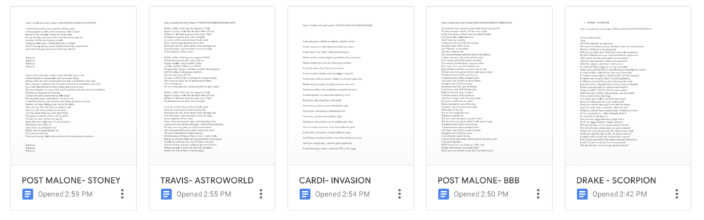
After looking through the different text-mining tools, I decided to use Voyant. I downloaded the cookbooks as .txt files and renamed them by their date of publication for a cleaner look. I uploaded the files and this is the breakdown of my corpus: https://voyant-tools.org/?corpus=b29265bf19df5fdf4ea6a0d11cc3c345&panels=cirrus,reader,trends,summary,contexts

The Summary tab gives an overview of the corpus: 7 documents with 381,754 total words and 9,972 unique word forms. The longest document is the 1896 cookbook at 151,148 words and the shortest is the 1798 cookbook at 14,800 words. The 1798 cookbook has the highest vocabulary density and the lowest density is the 1896 cookbook. The five most frequent words in the corpus are ‘water’ (3,074); ‘butter’ (2,481); ‘add’ (2,439); ‘salt’ (2,250); and ‘cup’ (2,224). I wanted to see more results, so I moved the ‘Items’ slide bar on the bottom and it gave me the top 25 most frequent words in the corpus. The above chart shows the Relative Frequency of the top five words. I found it interesting how often the word ‘cup’ was used throughout the corpus. In 1798 ‘cup’ was counted 6 times and ‘cups’ 8 times. In the 1909 cookbook, ‘cup’ was counted 516 times and ‘cups’ 158 times. Granted the 1909 text is much longer than the 1798 text (approximately 35,000 words more), but I wondered what measurement terms were used in 1798. I entered common terms, and saw that ‘pint’ was used 68 times, ‘quart’ 94 times ‘spoonful’ 9 times and ‘ounce’ 12 times in the 1798 cookbook. Interestingly enough, neither ‘teaspoon/s’ nor ‘tablespoon/s’ were used in the 1798 or 1803 cookbooks.
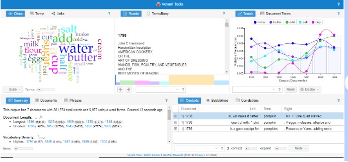
I then looked at common cooking terms and ran into my first issue. I know modern cooking terms, but what were common terms used in the 18th and 19th centuries? Looking at the word cloud Voyant produced helped, as well as the most frequent terms for each cookbook. After creating my initial list, I had to decide how I wanted to input the terms. Do I only include ‘sear’ or all words beginning with sear (‘sear*’) so I don’t miss terms in different tenses? When I just used ‘sear’ I had 5 counts, but ‘sear*’ is 15. I looked them up, and 18 ‘sear’ terms were cooking related (one was ‘sear’d’) and the other 2 instances were the word ‘search’. I’m sure that using all terms with an ‘*’ has skewed the results a bit, but as of right now I would rather be inclusive.
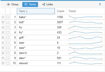
Next, I wanted to focus on food items, so I added measurements and related words to the list of stopwords. Added were: add, cup, tea/tablespoon, half, make, bake, pour, hot and dish. What showed up was slightly different, but I still saw some measurement terms and realized that I had to add the plural forms of words like tablespoon, cup, etc. I was thinking about removing ‘pound’ but there are recipes for pound cake and pear was called ‘Pound Pear’ (1798 cookbook) so I decided to keep it. After the words were added, the most common words in the corpus were: ‘water’ ‘flour’ ‘butter’ ‘sugar’ ‘milk’ and ‘eggs.’ I then looked at what meats were used and when. ‘Fish’ was the most popular, with ‘turkey’ and ‘pigeon’ at the bottom.
A side part of this project is to see when American cookbooks included what we think of as traditional Thanksgiving fare. I decided to look up pumpkin (pie), cranberry sauce and sweet potato. I also wanted to look up cocoa/chocolate. Looking up pumpkin was interesting. ‘Pumpkin’ was in every cookbook except in 1798. Through an internet search, I found out that pumpkin was spelled ‘pompkin’ at that time and once I searched the word, ‘pompkin’ is mentioned in the 1798 book 3 times. And it is for two variations of a pompkin pudding. By 1803, ‘pompkin’ was changed to ‘pumpkin’ and there was a recipe for a pie. Pumpkin came up the most in 1857. For cranberry, cranberries were first mentioned in 1803 for tarts. But over time cranberry sauce recipes were included. Sweet potatoes were first mentioned in 1838. Cocoa/ chocolate was first included in the 1838 cookbook.
Thoughts
I really enjoyed looking through the cookbooks, but I know that if I were to expand on this project, I would need to do more research about traditional cooking terms and recipes so I could get more accurate results. My current knowledge about this topic is not enough to make the decisions about what terms to focus on or what I can safely add to the list of stopwords. I would also need to find a larger collection of cookbooks. Feeding America was a great site for an introduction to text analysis, but there are only 76 cookbooks available, and some of them were more of a guide for women and the home than cookbooks. I need to look into how many cookbooks were actually published during this time. There were also books that focused on Swedish, German or Jewish-American cuisine, but they were published in the late 19th/early 20th centuries. I would like to investigate that topic further-when did ‘immigrant cookbooks’ first get published? Voyant was a good fit for this project, and I would recommend using it for those who are dipping their toes into text analysis. It was easy to upload the .txt files and fun to play around with the different Tools in each section (Scatter Plot, Mandala, etc). If I wanted to expand this project, I would have to investigate if Voyant would be as easy to use with a much larger corpus.
Towards a Text Analysis of Gender in the Psalms of Solomon
My initial intention for the Text Analysis praxis was to try to follow the procedure recommended by Lisa Rhody in the Text Analysis course I am taking this semester, as outlined in the article “How We Do Things With words: Analyzing Text as Social and Cultural Data,” by Dong Nguyen, Maria Liakata, Simon DeDeo, Jacob Eisenstein, David Mimno, Rebekah Tromble, and Jane Winters. https://arxiv.org/pdf/1907.01468.pdf. They identify five project phases (1) identification of research questions; (2) data selection; (3) conceptualization; (4) operationalization; (5) analysis and the interpretation of results.
1. Identification of Research Questions: I realized that my research aim was not really a question, but something more like: play around with text analysis.
2. Data Selection: To select my data, I decided to work with texts that I have worked on in my biblical research. I had initially thought to work with a legal term that appears in talmudic texts. I found an open access digitized corpus of the Talmud online (at https://www.sefaria.org/), but I lacked the programming skills to access the full corpus, scrape, and search it.
So I decided to work instead with the Psalms of Solomon– a collection of 18 psalms that is dated to the 2nd century B.C.E. I am currently writing an article based on a conference paper that I presented on gender stereotypes in the Psalms of Solomon. My delivered paper was highly impressionistic, and quite basic: introducing simple premises of gender-sensitive hermeneutics to the mostly-male group of conference participants. In selecting The Psalms of Solomon for this praxis, I can pull together my prior “close reading” research on this text, with the coursework for the 3 CUNY courses I am taking this semester: our Intro course; the “Text Analysis” course, in which the focus is “feminist text analysis”; and Computational Linguistics Methods 1.
Since the Psalms of Solomon is just a single document, with 7165 words (as I learned from Voyant, below), it does not lend itself to “distant reading”. I simply hoped it could serve as a manageable test-case for playing with methods.
For the Computational Linguistics course, I will work with the Greek text. (https://www.sacred-texts.com/bib/sep/pss001.htm
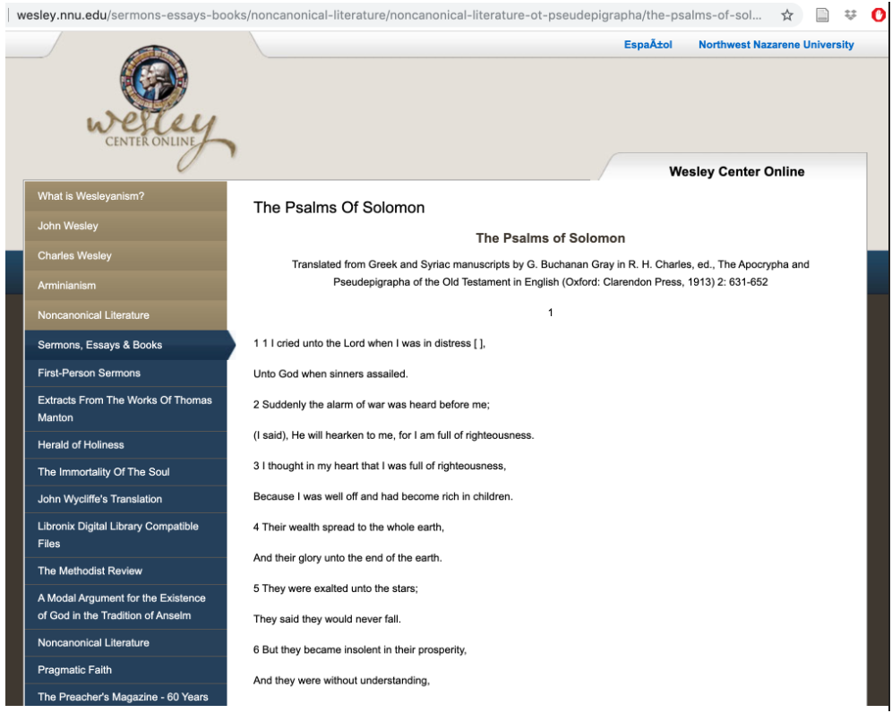
For our praxis, I thought it more appropriate to work with the English translation:
http://wesley.nnu.edu/sermons-essays-books/noncanonical-literature/noncanonical-literature-ot-pseudepigrapha/the-psalms-of-solomon/
(3) Conceptualization: since my main aim was to experiment with tech tools, my starter “concept” was quite simple: to choose a tool and see what I could do with the Psalms of Solomon with this tool.
(4) operationalization: After reading Amanda’s blog post about the Iliad, (https://dhintro19.commons.gc.cuny.edu/text-analysis-lessons-and-failures/) I mustered the courage to create a word cloud of PssSol with Voyant.
https://voyant-tools.org/?corpus=a748e4c58fbb317b36e0617bf8b61404

(5) analysis and the interpretation of results.
The most frequent words make sense for a collection of prayers with a national concern, and aligns with accepted descriptions of the psalms: “lord (112); god (108); shall (73); righteous (38); israel (33)”. The word “shall” is introduced in the English translation, since Greek verbal tenses are built in to the morphology of the verbs. I was pleasantly surprised to see that the word cloud reflects more than I would have expected. Specifically, it represents the dualism that is central to this work: the psalms ask for and assert the salvation of the righteous and the punishment of the wicked. I reduced the number of terms to be shown in the word cloud, and saw the prominence of “righteous”/”righteousness”, and “mercy”, as well as “pious”, and also “sinners”, though less prominently. In an earlier publication, I wrote about “theodicy” in the Psalms of Solomon– the question of the justness of God as reflected in divine responses to righteousness and evil.
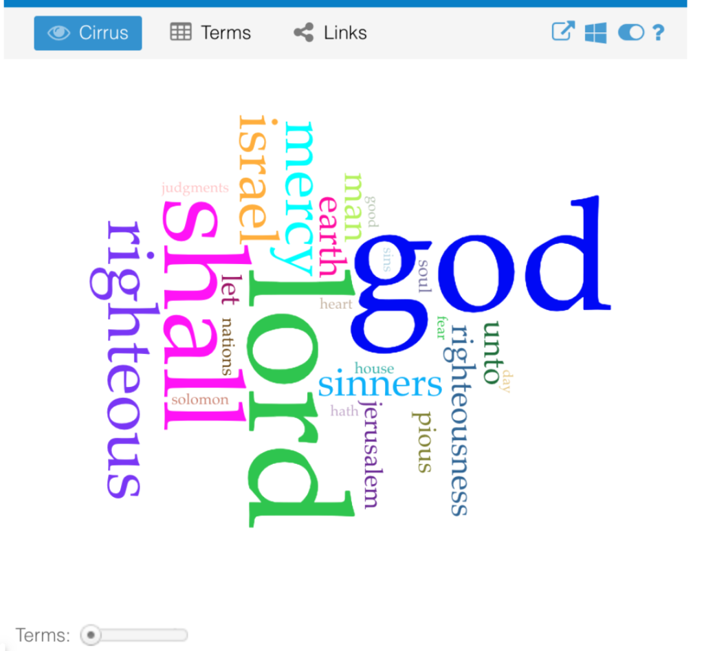
Viewing this visualization of the content of Psalms of Solomon with my prior publication in mind made me feel more comfortable about Voyant, even though it just displays the obvious.
Setting the terms bar to the top 95 words further strengthened some of my warm fuzzies for Voyant. Feeling ready to step up my game, I tried to return to Step 3, “Conceptualization.” I know I want to look at words pertaining to gender. But I find myself stuck as far as I can get with Voyant.
In the meantime, I’ve met with my Comp. Linguistics prof., and my current plan for that assignment is to seek co-occurrences for some some gendered terms: possibly, “man/men” (but this can be complicated, because sometimes “man” means male, and sometimes it means “person”, and, as is well-known, sometimes “person” sort of presumes a male person to some exgent); “women“, “sons” (again, gender-ambiguous), “daughters“; maybe verbs in feminine form.
At this point, I only reached the stage of accessing the source code, which, on my machine, I do as follows:
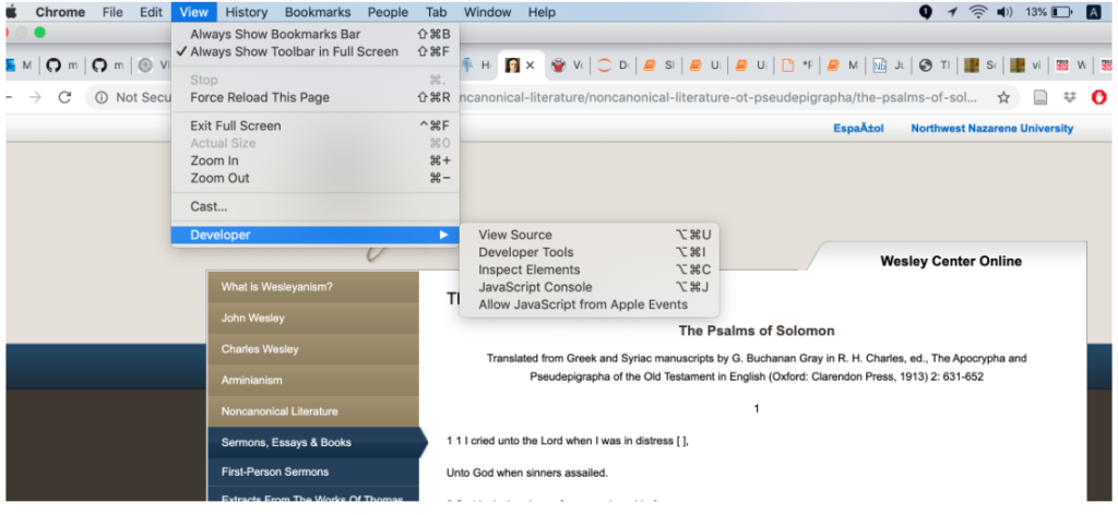
This yields:
I find this very exciting, especially the part that contains the text:

As it turns out, the code for the Greek is actually simpler than the code for the English:

I’m looking forward to working with this text, but this is as far as I’ve been able to get up to this point. My first task is to collect all of the 18 Psalms into a single file, by iterating over the URL, since the website for the Greek text has a separate page for each psalm. Then, I will think about what to search for, and how….
text messaging: not a hot new epistolary form
This project aims to make some meaning from over a quarter million text messages exchanged over the course of a 6+ year relationship. It is an extension of a more qualitative project I began in 2017.
Here’a a recap of Part I:
In the spring of 2017, I was a senior in college. My iPhone was so low on storage that it hadn’t taken a picture in almost a year, and would quit applications without warning while I was using them (Google Maps in the middle of an intersection, for example). I knew that my increasingly lagging, hamstringed piece of technology was not at the necessary end of its life, but simply drowning in data.
The cyborg in me refused to take action, because I knew exactly where the offending data was coming from: one text message conversation that extended back to 2013, which comprised nearly the entire written record of the relationship I was in, and which represented a fundamental change in the way I used technology (spoiler: the change was that I fell in love and suddenly desired to be constantly connected through technology, something I had not wanted before). And in the spring of 2017, I didn’t want to delete the conversation because I was anxious about whether the relationship would continue after we graduated college.
Eventually, though, I paid for a software that allowed me to download my text messages and save them as .csv, .txt, and .pdf on my computer. (I also saved them to my external hard drive, because in addition to not knowing if my relationship would survive the end of college, I also had no job offers and was an English major and I really needed some reassurance.) So I did all of that, for all 150,000+ messages and nearly 3GB worth of [largely dog-related] media attachments. This is but one portrait of young love in the digital age.
I wrote a personal essay about the experience in 2017, which focused on the qualitative aspect of this techno-personal situation. Here is an excerpt of my thoughts on the project in 2017:
“I was sitting at my kitchen table when I downloaded the software to create those Excel sheets, and I allotted myself twenty minutes for the task. Four and a half hours later, I was still sitting there, addicted to the old texts. Starting from the very beginning, it was like picking up radio frequencies for old emotions as I read texts that I could remember agonizing over, and texts that had made my heart swell impossibly large as I read them the first time. …
I had not known or realized that every text message would be a tiny historical document to my later self, but now that I had access to them going all the way back to the beginning, they were exactly that to me as I sat poring over them. It was archaeology to reconstruct forgotten days, but more often than not I was unable to reconstruct a day and just wondered what we had done in the intervening radio silences that meant we were together in person. These messages made the negative space of a relationship, and the positive form was not always distinguishable in unaided memory. “
The piece concluded with a reminiscence of a then-recent event, in which a friend of ours had tripped and needed a ride to the emergency room at 3 in the morning. We were up until 5am and ended up finishing the night, chin-stitches and all, at a place famous for opening for donuts at 4 in the morning. The only text message record of that now oft-retold story is one from me at 3:45am saying “How’s it going?” from the ER waiting room, and a reply saying “Good. Out soon”. I concluded that piece with the idea that while the text message data was powerful in its ability to bring back old emotions and reconstruct days I would have otherwise forgotten, it was obviously incomplete and liable to leave out some of the aspects most important to the experiences themselves.
So now, Part II of this project.
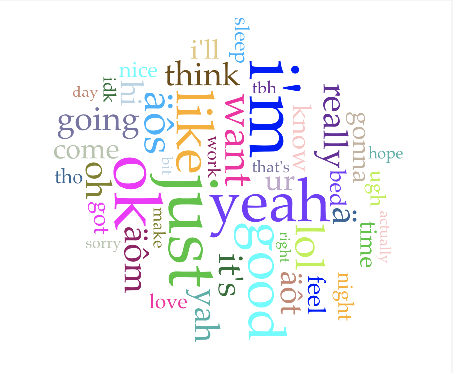
I compiled a new data set, taken from the last two years of backups I have done with the same software (and same relationship — we have thus far lasted beyond graduation). I loaded the data into Voyant, excited to do some exploratory data analysis. The word cloud greeted me immediately, and I thought to myself “is this really how dumb I am?”
Okay, maybe that’s a bit harsh, but truly, parsing through this data has made me feel like I spend day after day generating absolute drivel, one digital dumpster after another of “lol,” “ok,” “yeah,” “hi,” “u?” and more. I was imagining that this written record of a six year relationship would have some of the trappings of an epistolary correspondence, and that literary bar is 100% too high for this data. See the word cloud below for a quick glimpse of what it’s like to text me all day.
Some quick facts about the data set:
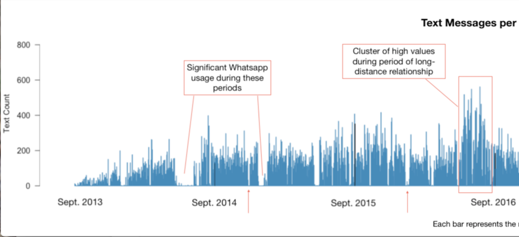
Source: all iMessages and text messages exchanged between August 31, 2013 and November 12, 2019, except a missing chunk of data from a 2-month lost backup (12-25-18 to 03-01-18). *****EDIT 11/19: I just found it!! iMessages switched from phone number to iCloud account, so were not found in phone number backup. Now there are just 18 days unaccounted for. As of now, the dataset still excludes WhatsApp messages, which has an impact on a few select parts of the dataset at times when that was our primary means of text communication (marked on the visualization below), but has relatively little impact overall.
The data set contains 294,065 messages total, exchanged over 6+ years. It averages out to 130.9 messages per day (including days on which 0 messages were sent, but excluding the dates for which there is no data). As per Voyant, the most frequent words in the corpus are just (23429); i’m (19488); ok (17799); like (13988); yeah (13845). The dataset contains 2,047,070 total words and 35,407 unique words. That gives it a stunningly low vocabulary density of 0.017, or 1.7%.
Counting only days where messages were exchanged, the minimum number of messages exchanged is 1 — this happened on 29 days. The maximum number of messages exchange in one day is 832. (For some qualitative context to go with that high number: it was not a remarkable day, just one with a lot of texting. The majority of those 832 messages were sent from iMessage on a computer, not a phone, which makes such a volume of messages more comprehensible, thumb-wise. I reread the whole conversation, and there were two points of interest that day that prompted lots of messages: an enormous, impending early-summer storm and ensuing conversation about the NOAA radar and where to buy umbrellas, and some last-minute scrambling to find an Airbnb that would sleep 8 people for less than $40 a night.)
I was curious about message counts per day — while it’s definitely more data viz than text analysis, I charted messages per day anyway, and added some qualitative notes to explain a few patterns I noticed.

Chopped in half so that the notes are readable:

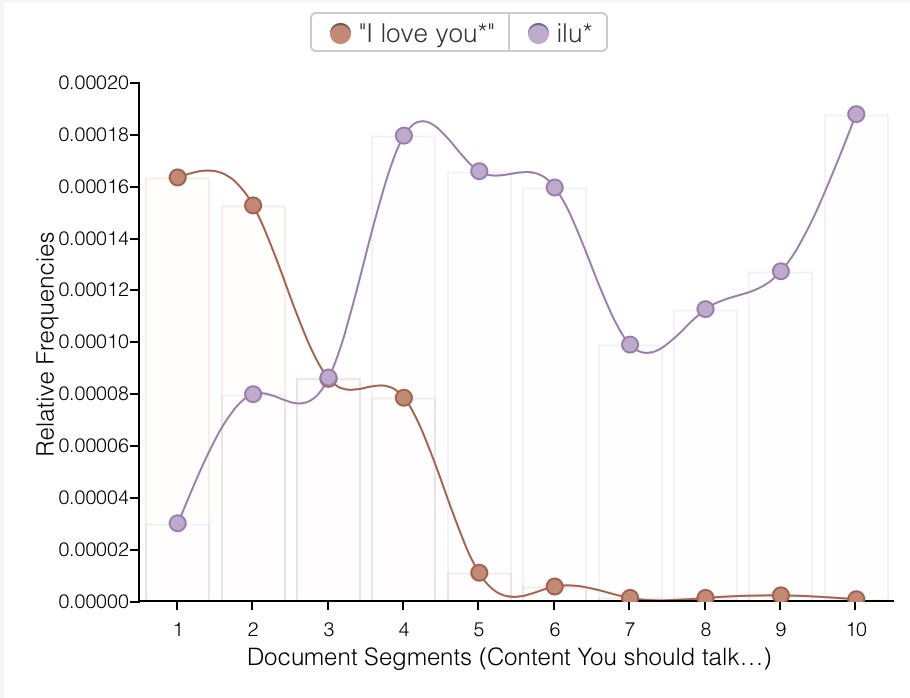
Despite my mild horror at the mundanity and ad nauseam repetition of “ok” and “lol,” I had fun playing around with different words in Voyant. I know from personal experience, and can now show with graphs, that we have become lazier texters: note the sudden replacement of “I love you” with “ilu” and the the rise of “lol,” often as a convenient, general shorthand for “I acknowledge the image or anecdote you just shared with me.”

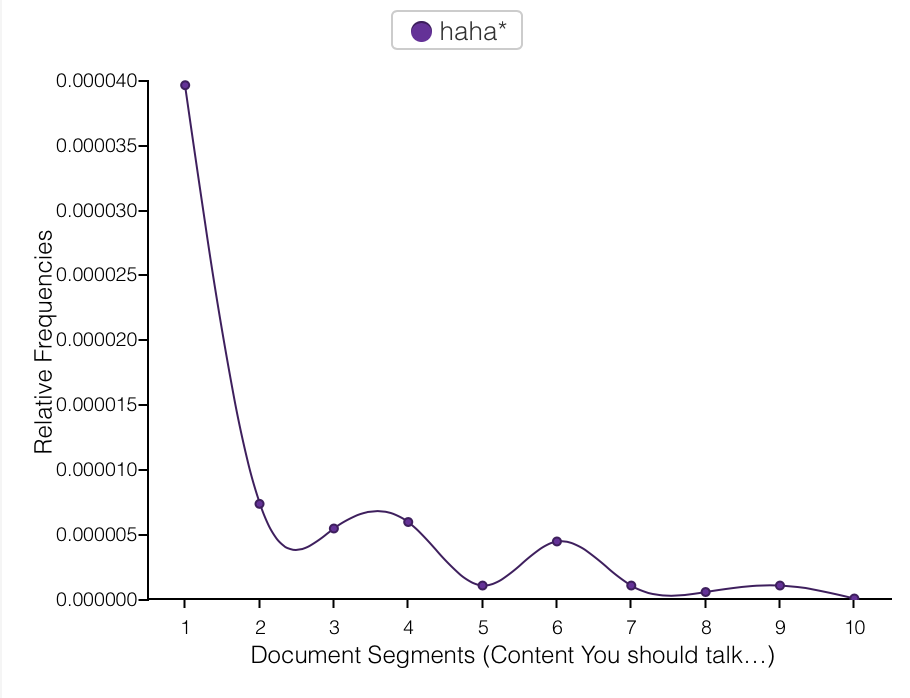
On the subject of “lol,” we have the lol/haha divide. Note the inverse relationship below: as “lol” usage increases, “haha” use decreases. (The two are best visualized on separate charts given that “lol” occurs more than 10 times as frequently as “haha” does.) I use “haha” when I don’t know people very well, for fear that they may feel, as I do, that people who say “lol” a lot are idiots. (“Lol” is the seventh most frequently used word in this corpus.) Once I have established if the person I’m texting also feels this way, i.e. if they use “lol,” I begin to use it or not use it accordingly. Despite this irrational and self-damning prejudice I have against “lol,” I use it all the time and find it to be one of the most helpful methods of connoting tone in text messages — much more so than “haha”, which may explain my preference for “lol”. “You are so late” and “You are so late lol” are completely different messages. But I’m getting away from the point… see “lol” and “haha” graphed below.

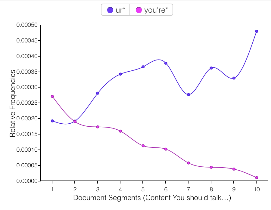
The replacement of “you” with “u,” however, I do not interpret as laziness, or as personal preference winning out, but as a form of ironical love language. At some point over the narrative span of this corpus, using “u” was introduced as a joke, because both of us were irked by people texting w/o putting any effort in2 their txts bc it makes it rly hard 2 read n doesnt even save u any time 2 write this way? And then it turned out it maybe does save a tiny bit of time to write “u” instead of “you,” and more importantly “u” began to mean something different in the context of our conversations. Every “u” was not just a shortcut or joke, but had, with humorous origins, entered our shared vocabulary as a now-legitimate convention of our communal language. Language formation in progress! “Ur” for “you’re” follows the same pattern.

With more time, I would like to evaluate language from each author in this corpus. It is co-written (52% from me, 48% to me) and each word is directly traceable back to one author. Do we write the same? Differently? Adopt the same conventions over time? My guess is that our language use converges over time, but I didn’t have time to answer that question for this project.
I began this text analysis feeling pretty disappointed with the data. But through the process of assigning meaning to some of the patterns I noticed, I have come to appreciate the data more. I also admit to myself that once I had the thought that text messaging– writing tiny updates about ourselves to others– is a modern epistolary form, I perhaps subconsciously expected it to follow in the footsteps of Evelina… which is an obviously ridiculous comparison to draw. Or for it to evoke to some extent the letters written between my grandparents and great-grandparents, which is a slightly less ridiculous expectation but one that was still by no means lived up to. Composing a letter is a world away from composing a text message. Editing vs. impulse. Text messages are “big data” in a way that letters will never be, regardless of the volume of a corpus.
Would it be fascinating or incredibly tedious to read through your grandparents’ text conversations? Probably a bit of both, satisfying in some ways and completely insufficient in others. It’s not a question that we can answer now, but let’s check again in fifty years.

JSTOR Text Analyzer
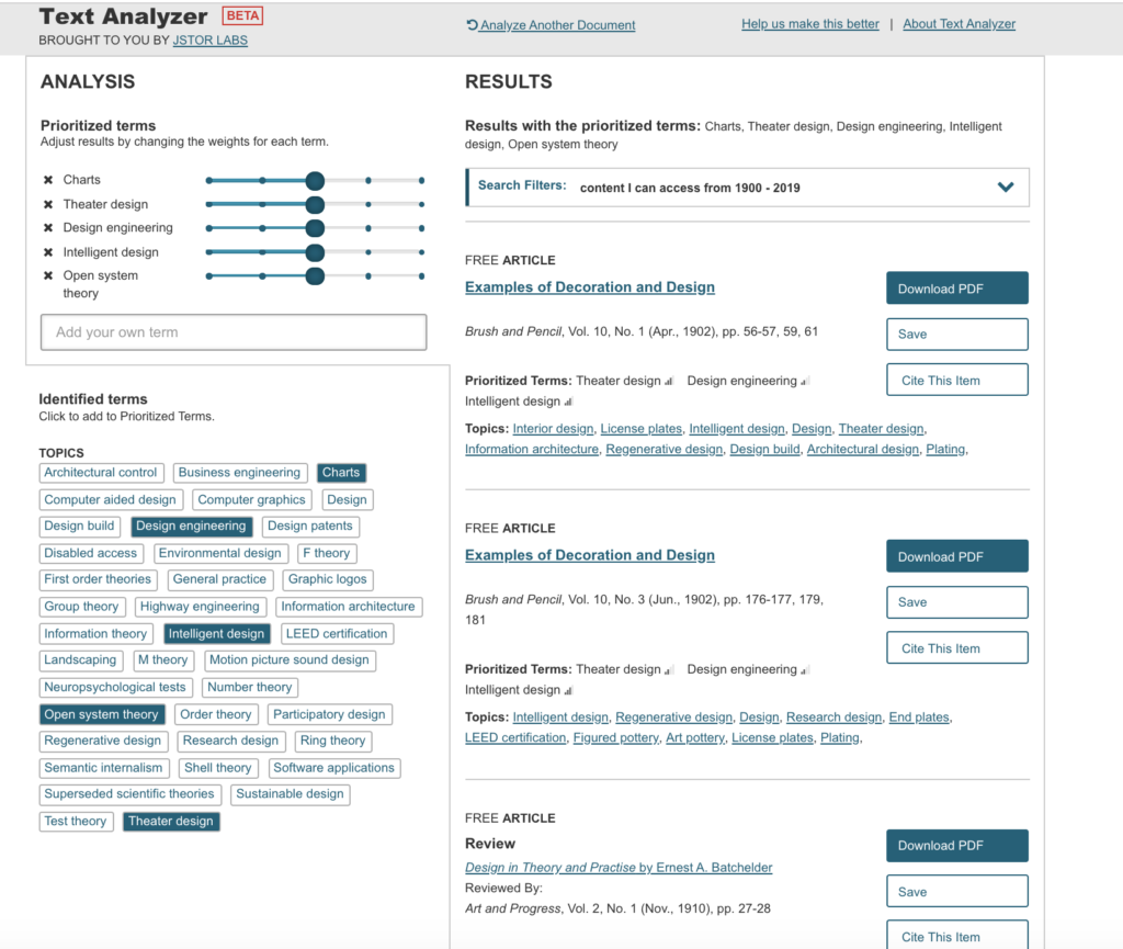
When I began this text analysis praxis, I thought I might try out one of the flashier tools in the list, maybe Voyant, Google N-Gram, or MALLET (which I did end up playing around a bit with, but ran out of time trying to find all the texts I wanted to build a decent sized corpus). I had hoped to end up with some interesting findings or at least some impressive images to share with you on this blog post! What I did decide on was the JSTOR Text Analyzer, definitely the least sexy option in the list, but for me, probably the most useful tool for my daily work as a librarian.
I will be completely honest and say that I am not a fan of paywalls and the companies that build them, that being said, many academic institutions subscribe to JSTOR and as an academic librarian I need to understand what are the tools that can best help library patrons. Using the Text Analyzer tool is simple, nothing to download, no code to write, you just upload a document with text on it, (they say even if it is just a picture of text) and the tool will analyze it and find key topics and terms, then you get to prioritize these terms, change the weight given to them in the search and use them to find related JSTOR content.
This all seems simple enough, they say they support a whole slew of file types (csv, doc, docx, gif, htm, html, jpg, jpeg, json, pdf, png, pptx, rtf, tif (tiff), txt, xlsx) and fifteen (!) languages including: English, Arabic, (simplified) Chinese, Dutch, French, German, Hebrew, Italian, Japanese, Korean, Polish, Portuguese, Russian, Spanish and Turkish. And as a bonus, they will even help you find English-language content if your uploaded content is in a non-English language. This all sounded too good to be true, so I thought I would go real-world and drop in a bunch of real syllabi (see course list below) from professors I have helped this semester and see how the JSTOR Text Analyzer would score.
Courses
- Philosophy of Law (Department of Social Science)
- Building Technology III (Department of Architectural Technology)
- Information Design (Department of Communication Design)
- Sustainable Tourism (Department of Hospitality Management)
- Electricity for Live Entertainment (Department of Entertainment Technology)
- Hospitality Marketing (Department of Hospitality Management)
The Process
The first course I tried was Philosophy of Law. I used the “Drag and Drop” feature to upload a pdf of the course syllabus. Once the file is “dropped” into the search box, the JSTOR Text Analyzer takes over and produces results in seconds. This is what my first search produced. The results were somewhat relevant to the course and not too bad for a first try. At this point I decided to add a few terms from the syllabus and change the weight that those terms are given in the search.
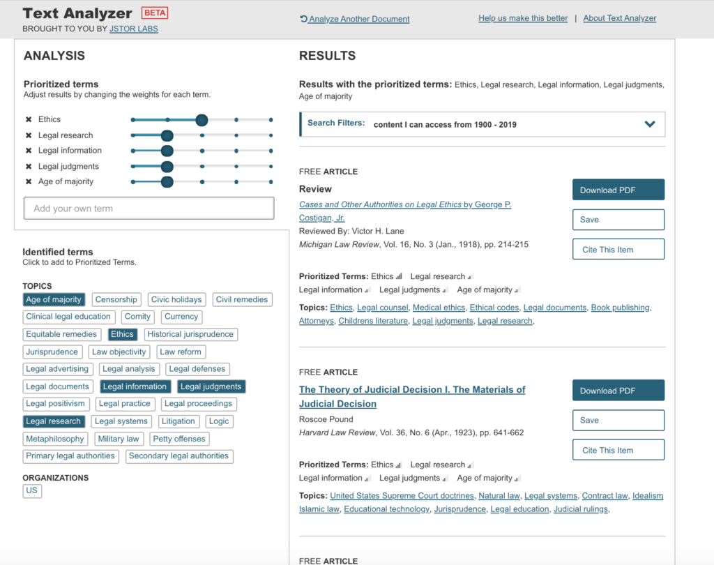
Here are the results of my second, modified search.

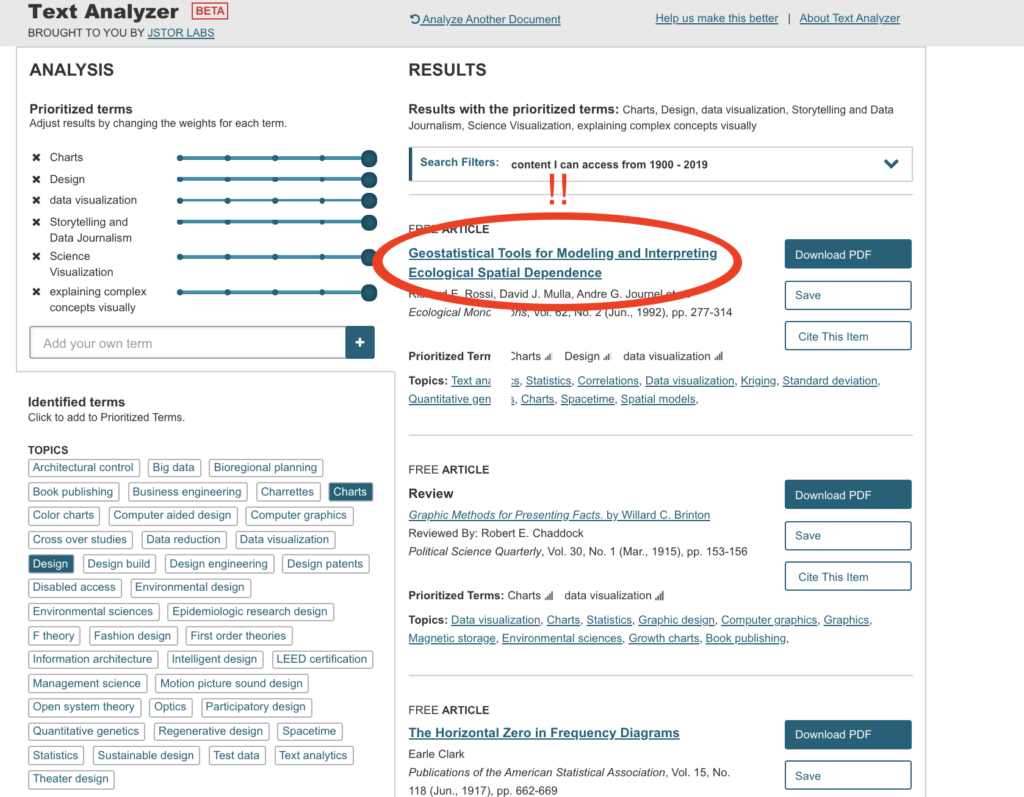
Next I uploaded a csv file of a syllabus for Building Technology III. The Text Analyzer had no problem with the change in file format. The search results for this course were a bit strange though, with an article about the Navy’s roles and responsibilities in submarine design being the first in my results list. I am not sure where the JSTOR algorithm inferred the military and submarine from as there was nothing in the syllabus that made reference to these subjects. Oh the mysteries of the “black box algorithm”.

I then did the same addition and deletion of terms and adjusted term weights as I did for the previous course, Philosophy of Law. The new search results were much closer to the actual course content, though I did expect to see more about steel.

For my next experiment, I chose to take a screenshot of the syllabus for Information Design and import the png image file into the Text Analyzer. Unfortunately, even though they say they support png files, I received the following when I uploaded mine.
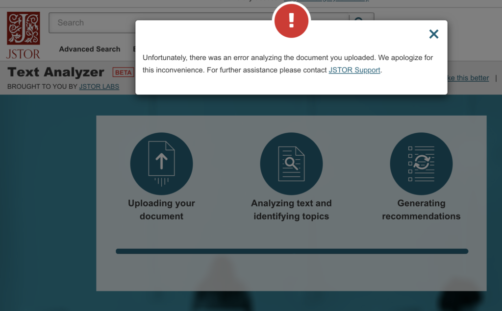
File types supported
https://www.jstor.org/analyze/about
You can upload or point to many kinds of text documents, including: csv, doc, docx, gif, htm, html, jpg, jpeg, json, pdf, png, pptx, rtf, tif (tiff), txt, xlsx. If the file type you’re using isn’t in this list, just cut and paste any amount of text into the search form to analyze it.
I then went back to uploading pdfs and did not have any further problems with importing the syllabus for Information Design. The initial search results were not bad and actually got worse when I modified the terms to reflect what was in the syllabus.
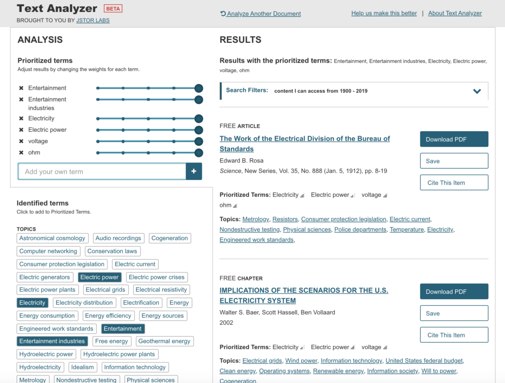
The syllabus for Electricity for Live Entertainment uploaded with no problems and the results were interesting and made reference to electricity but not entertainment.
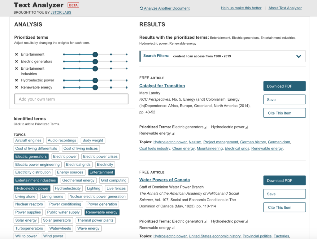
The modified results were far more relevant to the course content.
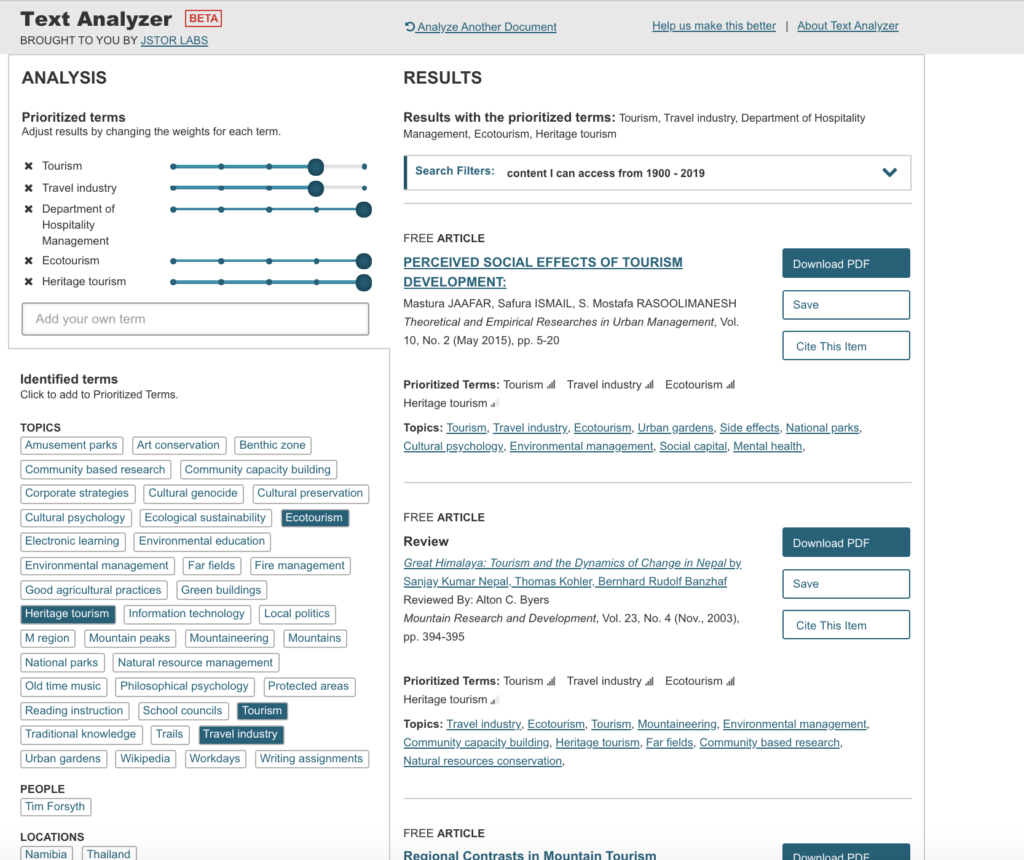
I then moved on the Sustainable Tourism. Things went really weird when I tried to upload a url for a course website that contained the syllabus (all these are Open Educational Resource – OER – courses) and the Text Analyzer picked up some crazy stuff, maybe from the metadata of the website itself??

I then uploaded the syllabus directly, as a pdf and received pretty accurate search results.
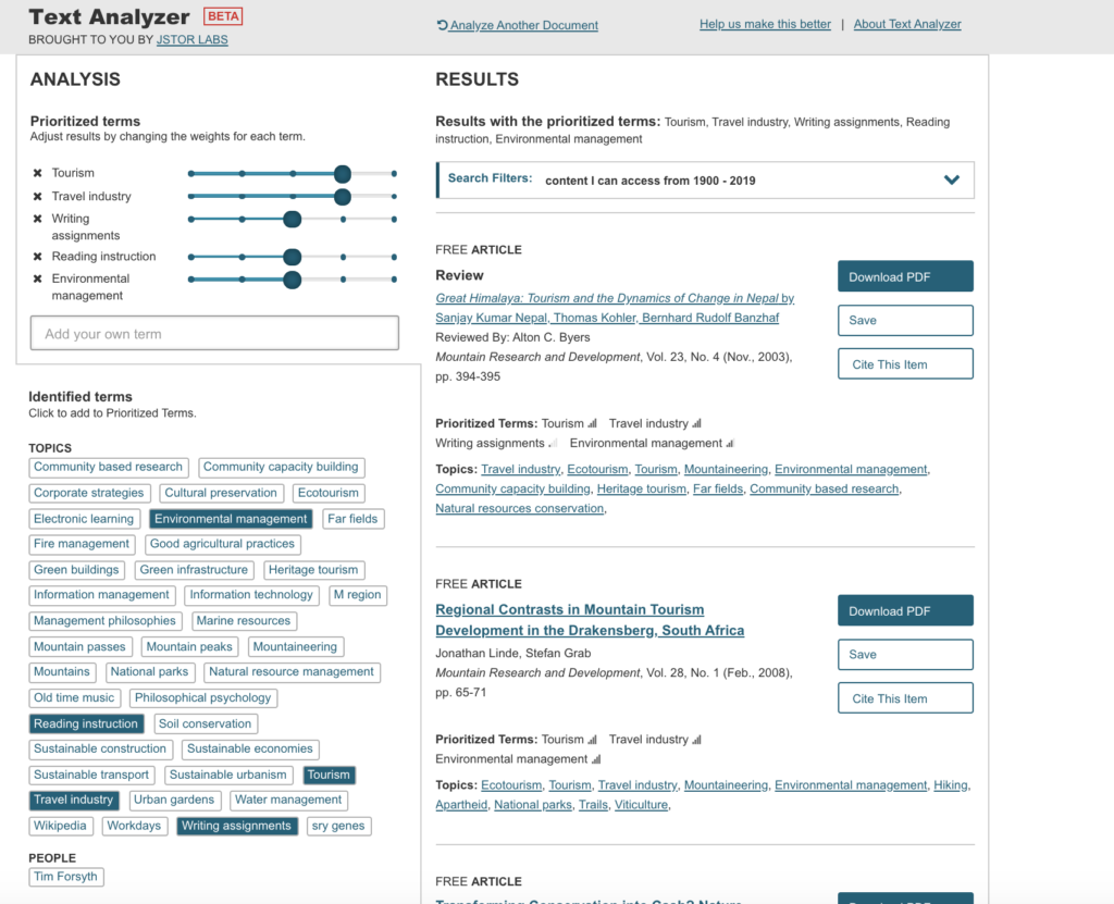
Modified results for Sustainable Tourism were even better.
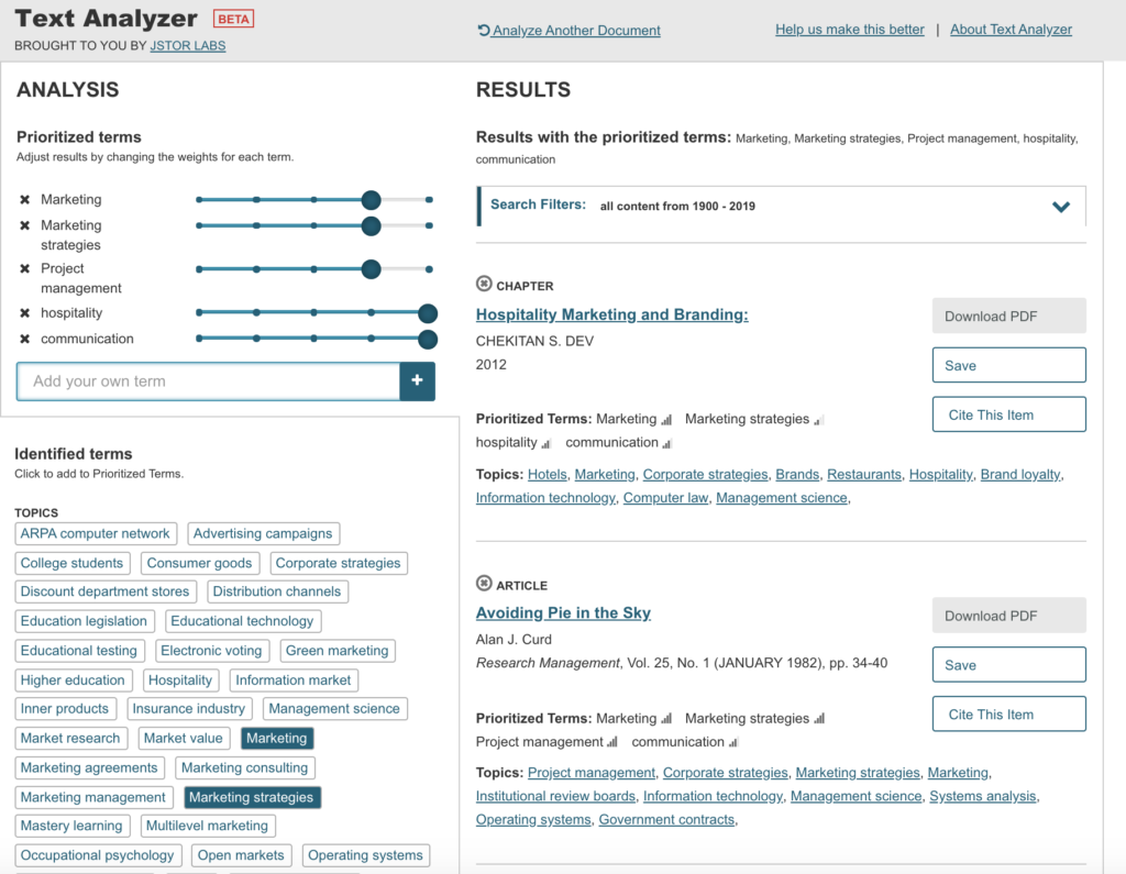
The search results for Hospitality Marketing, upload by pdf, were completely off, not even close.
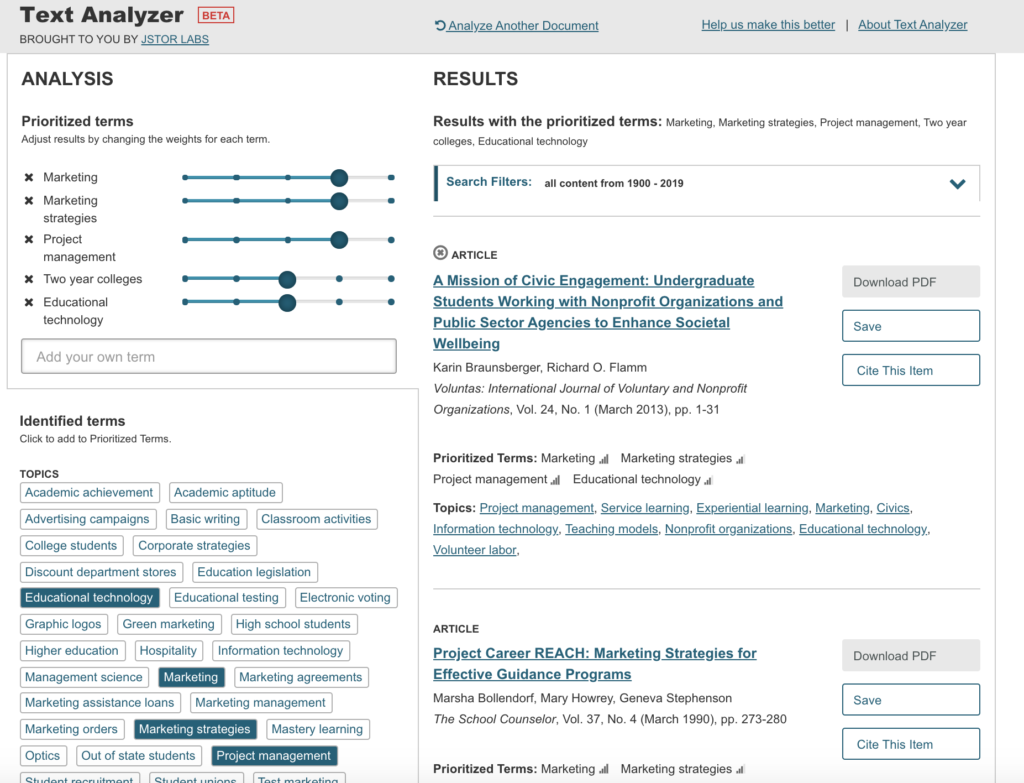
Modified terms and weights gave me much better and more accurate results.
My Thoughts
In the end, the JSTOR Text Analyzer is not a bad tool for finding content based on textual analysis of an imported file. Upload is simple and the results, while mixed, are generally in the ballpark. Adjustment of terms and weight is almost alway necessary, but not difficult to do. I probably use and recommend this tool. I did not log in and instead used the “open” version of content, but if you have access to JSTOR content through your institution, you would probably get different and maybe even better results.
And because no text analysis project is complete without a world cloud, here is one I made using text from all the syllabi I uploaded into the JSTOR Text Analyzer.

OMG! TF-IDF!
New to quantitative text analysis, I began this assignment with Voyant and Frederick Douglass’s three autobiographies. Not only are the texts in the public domain, but their publishing dates (1845, 1855, and 1881) punctuate the nation’s history that he helped shape across years that saw the passage of the Fugitive Slave Act of 1850, the Civil War, and Reconstruction.
Voyant’s instant and multi-pronged approach was exciting. A superficial glance confirmed what I expected: each text is substantially larger than the former, and terms describing enslavement are most frequent. I played around, loving particularly the MicroSearch (because it reminded me of a dynamic viz of Darwin’s revisions of Origin of the Species) and the animated DreamScape.

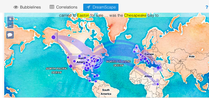
But, I saw clear errors that I couldn’t correct on this side of what Ramsay and Rockwell referred to as the “black box.” In DreamScape, “Fairbanks” had been misread as the name of the Alaskan city rather than a man who drives Douglass out of a school in St. Michael’s. The widget did allow me to view the text references it had mapped—a helpful peek under the hood—but without an option to remove the errant attribution. I remembered Gil’s suspicion in “Design for Diversity” of programs like Voyant. He warned that “use of these tools hides the vectors of control, governance and ownership over our cultural artifacts.” Particularly given the gravity of the subject of enslavement in the texts I was exploring, I thought I’d better create my own interpretive mistakes rather than have them rendered for me.
In last spring’s Software Lab, I’d had a week or two with Python, so I thought I’d try to use it to dig deeper. (The H in DH should really stand for hubris.) I read a little about how the language can be used for text analysis and then leaned heavily on a few online tutorials.
I started by tokenizing Douglass’s words. And though my program was hilariously clumsy (I used the entire text of each autobiography as single strings, making my program tens of thousands of lines long), I still was thrilled just to see each word and its position print to my terminal window.
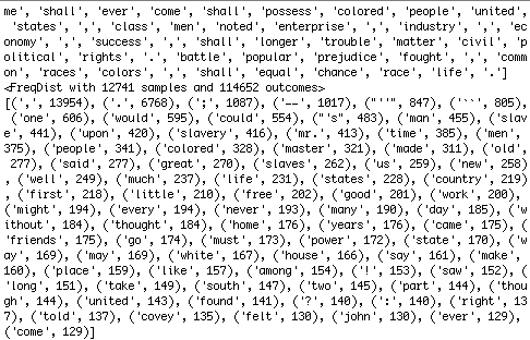
I then learned how to determine word frequencies. The top 20 didn’t reveal much except that I had forgotten to exclude punctuation and account for apostrophes—something that Voyant had done for me immediately, of course. But, because my code was editable, I could easily extend my range beyond the punctuation and first few frequent terms.
from nltk.probability import FreqDist
fdist = FreqDist(removing_stopwords)
print(fdist)
fdist1 = fdist.most_common(20)
print(fdist1)
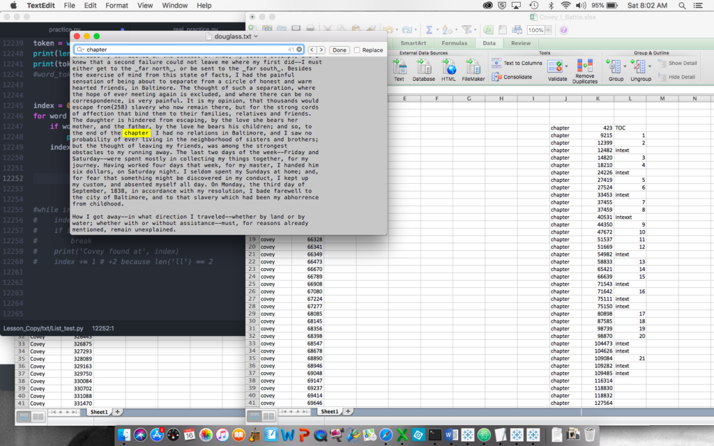
So, I bumped 20 to 40, 40 to 60, and 60 to 80, when something interesting happened: the appearance of the name Covey. Despite my sadly eroding familiarity with Douglass’s life, I remembered Covey, the “slave breaker” whom enslavers hired when their dehumanizing measures failed to crush their workers’ spirits, and the man whom Douglass reports having famously wrestled and beat in his first physical victory against the system.
Excited by the find, I wanted to break some interesting ground, so I cobbled together a program that barely worked using gensim to compare texts for similarity. Going bold, I learned how to scrape Twitter feeds and compared Douglass’s 1855 text to 400 #BlackLivesMatter tweets, since his life’s work was dedicated to the truth of the hashtag. Not surprisingly given the wide gulf of time, media, and voice, there was little word-level similarity. So, I tried text from the November 1922 issue of The Crisis, the NAACP’s magazine. Despite the narrower gap in time and media, the texts’ similarity remained negligible. Too many factors complicated the comparison, from the magazine’s inclusion of ads and its poorly rendered text (ostensibly by OCR) to perhaps different intended audiences and genres.
Finally, I happened on “term frequency – inverse document frequency” (tf-idf)—a formula built to calculate the significance of words in a given text within a corpus by considering their frequency within that document and lack of it in the others. The Programming Historian offered a great tutorial using a range of obituaries from the New York Times as the corpus. Unfortunately for me, there were two errors in the code which took hair-pulling hours and a visit to the Python Users Group at CUNY to figure out. (I learned a brilliant and probably super obvious troubleshooting technique: when the line reference in the error doesn’t help, include print commands after chunks of code to see where the program is really breaking down.)
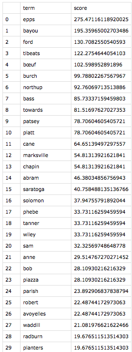
Eager to use my program on texts I chose, I returned to Douglass. Thanks to serendipity, I learned that Solomon Northup’s Twelve Years a Slave was published in 1853, just two years before Douglass’s second autobiography, My Bondage and My Freedom. My program, in thrilling seconds, spit out tf-idf findings of each document within the context of them together.
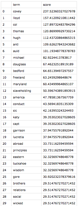
Both to make meaning out of the results and to make sure I wasn’t making errors like Voyant misreading Fairbanks, I investigated the instances of each of the top 21 words for each text. (Yes, I made the classic error of forgetting that index positions start with zero, so I focused on 0 – 20, not realizing that I was looking at 21 terms in each list.) In “All Models Are Wrong,” Richard Jean So had mentioned, “Perhaps the greatest benefit of using an iterative process is that it pivots between distant and close reading. One can only understand error in a model by analyzing closely the specific texts that induce error; close reading here is inseparable from recursively improving one’s model.” So, as distant reading led to close reading, exciting patterns across these two narratives emerged.
While the top 21 terms are unique to each text, these results share categories of terms. The highest-ranked term for each narrative is an ungodly cruel white man–Covey for Douglass, and Epps for Northup. Also statistically significant are enslavers whom the authors deem “kind,” geographical locations that symbolize freedom, stylistic terms unique to each author, and terms that are inflated by virtue of having more than one meaning in the text. I arrived at these categories merely by reading the context of each term instance—a real pleasure.
In digging in, I came to appreciate Douglass’s distinctive rhetorical choices. Where both authors use the term “slavery,” only Douglass invokes at high and unique frequency the terms “anti-slavery” and “slaveholding”—both in connection to his role, by 1855, as a powerful agent for abolition. The former term often refers quite literally to his career, and he uses the latter, both as an adjective and gerund, to distinguish states, people, and practices that commit to the act of enslavement. Like the term “enslaver,” Douglass charges the actor with the action of “slaveholding”—a powerful reminder to and potential indictment of his largely white audience.
I was most moved by the presence on both lists of places that symbolize hope. The contrasts of each author’s geographic symbols of freedom highlight the differences in their situations. Stolen from New York to be enslaved in far off Louisiana, Northup’s symbol of freedom is Marksville, a small town about 20 miles away from his plantation prison. A post office in Marksville transforms it in the narrative to a conduit to Saratoga, Northup’s free home, and thus the nearest hope. By contrast, Douglass, born into enslavement in Maryland, was not only geographically closer to free states, but he also frequently saw free blacks in the course of his enslavement. Making his top 21 includes nearby St. Michael’s, a port where he saw many free black sailors who, in addition to their free state worked on the open seas—a symbol of freedom in its own right. He also references New Bedford, Massachusetts, his first free home, like Northup’s Saratoga. America also makes his list, but Douglass invokes its promise rather than its reality in 1855—again perhaps more a choice for his white readers than for a man who, at this point, had never benefited from those ideals.
This distant-to-close reading helped bring to my consciousness the inversion of these men’s lives and the structure of their stories. For the bulk of their autobiographies, Northup moves from freedom to bondage, Douglas from bondage to freedom.
Given the connections between the categories of these unique terms, I was eager to “see” the statistics my program had produced. I headed to Tableau, which I learned in last summer’s data viz intensive.
After a lot of trial and error, I created what I learned is a diverging bar chart to compare the lists with some help from this tutorial. The juxtaposition was fascinating. Northup’s top terms mirrored those we’d see in the tale of any epic hero: helpers (both black and white) and myriad obstacles including the capitalized Cane, the crop that at this point ruled Louisiana. Further, his list includes his own names, both free (Solomon and Northup) and forced on him in enslavement (Platt), as if he needs to invoke the former as a talisman against the latter, textually reasserting his own humanity.
By contrast, Douglass’s top 21 is filled nearly exclusively with the men and women of the white world, whether foes or “friends.” His own names, enslaved or chosen, recede from his list (the appearance of Douglass on it is largely from the introductory material or references he makes to the title of his first autobiography).
Given Douglass’s patterns, I wanted to visualize his articulation of his struggle to claim himself against the soul-owning white world he was forced to serve. So, I adapted my Python tokenizing program to search for the location of the occurrences of “Covey” and “I” for Douglass and “Epps” and “I” for Northup. (I left alone the objective and possessive first-person pronouns, though I’d love to use the part-of-speech functions of NLTK that I’ve now read about.) This was the first program I created that had multiple uses: I could search the location of any term throughout the text. In addition to those I wanted to map, I also pulled the location of the word “chapter” so I could distribute the term locations appropriately into more comprehensible buckets than solely numbers among thousands. This required some calculated fields to sort list locations between first and last words of chapters.
I never quite got what I was looking for visually.* But analytically, I got something interesting through a stacked bar chart.

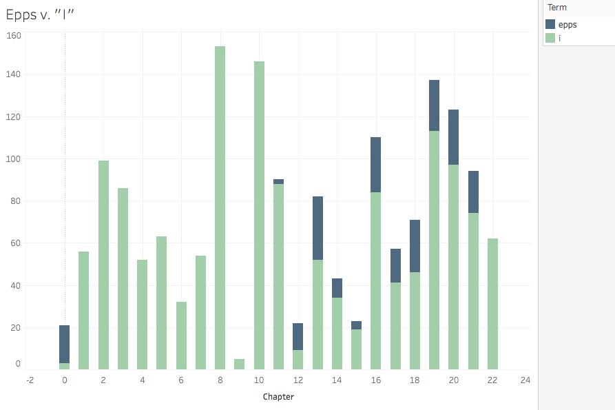
These charts suggest that Douglass’s battle with the cruelest agent of the cruelest system is fierce and fairly central—a back in forth of attempted suppression, with Douglass winning in the end. Nearly 500 self-affirming subject pronouns proclaim his victory in the penultimate chapter. Northup’s battle is far more prolonged (Epps is, after all, his direct enslaver rather than Covey who is more episodic for Douglass), and though he ends up victorious (both in the Epps/I frequency battle and in the struggle for emancipation), Epps lingers throughout the end of the narrative. I purposefully placed the antagonists on the top of the stack to symbolize Covey and Epps’ attempts to subjugate these authors.
As I’ve reviewed my work for this write-up, I’m hoping Richard Jean So will be pleased to hear this: my models are fraught with error. I should have been more purposeful in what counted as the text. Aside from the introductory material in chapters that I designated as 0, I did not think through the perhaps misleading repetition of terms natural in tables of contents and appendices. Also, by focusing on the top terms of the tf-idf calculations, I missed errors obvious had I looked at the bottom of the list. For example, while tokenizing, I should have accounted for the underscores rife in both texts, particularly in the tables of contents and chapter introductions, which might have changed the results.
The exercise also raised myriad questions and opportunities. I find myself wondering if Northup, upon regaining his freedom, had read Douglass’s first autobiography, and if Douglass had read Northup’s before writing his second. I think tf-idf is intended to be used across more than just two documents, so I wonder how these accounts compare to other narratives of enslavement or the somewhat related experiences of abduction or unjust imprisonment. Even within this two-text comparison, I’d like to expand the scope of my analysis past the top 21 terms.
Opportunities include actually learning Python. Successes still feel accidental. I’d like to start attending the Python User’s Group more regularly, which I might be able to pull off now that they meet Friday afternoons. My kindergarten skills for this project led to lots of undesirable inefficiency (as opposed to the great desirable inefficiency that leads to some marvelous happenstance). For example, I named my Python, Excel, Word, and Tableau files poorly and stored them haphazardly, which made it tough to find abandoned work once I learned enough to fix it. I’d also really love to understand file reading and writing and path management beyond the copy-from-the-tutorial level.
Regardless, I’m convinced that, for the thoughtful reader, distant reading can inform and inspire close reading. In fact, I’ve got a copy of the Douglass in my backpack right now, lured as I’ve become by the bird’s eye view.
*The area chart below of the terms Epps and I in the Northup is closer to what I wanted from a design perspective—the depiction of friction and struggle—but it’s not great for meaning, as the slope between points are fillers rather than representations of rises in frequency over time.
